在上一篇博客中，我们完成了一个简单的前馈神经网络，完成了对根据身高体重对性别进行猜测的神经网络，以及对他的训练。但是我们不该止步于此，接下来我们将尝试编写一个RNN循环神经网络，并认识它背后的原理。

循环神经网络简介

循环神经网络是一种专门用于处理序列的神经网络，因此其对于处理文本方面十分有效。且对于前馈神经网络和卷积神经网络，我们发现：它们都只能处理预定义的尺寸——接受固定大小的输入并产生固定大小的输出。但是循环神经网络可以处理任意长度的序列，并返回。它可以是这样的：

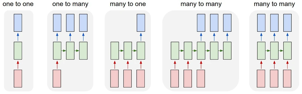
这种处理序列的方式可以实现很多功能。例如，文本翻译，事件评价… 我们的目标是让它完成对一个评论的判断（是正面的还是负面的）。将待分析的文本输入神经网络然后，然后给出判断。

实现方式

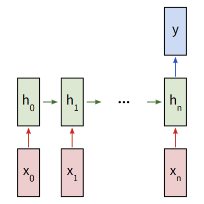
我们考虑一个输入为x0,x1,x2,...,xn，输出为y0,y1,y2,..,yn的多对多循环神经网络。这些xi和yi是向量，可以是任意维度。RNNs通过迭代更新一个隐藏状态h，重复这些步骤：

• 下一个隐藏状态h~t~是前一个状态h~t-1~和下一个输入x~t~计算得出的
• 输出y~t~是由当前的隐藏状态h~t~计算得出的

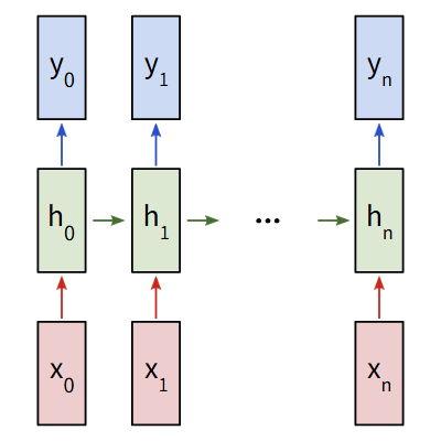
这就是RNNs为什么是循环神经网络的原因，对于上面步骤的每一步中，都使用的是同一个权重。对于一个典型的RNNs，我们只需要使用3组权重就可以计算：

• W~xh~ 用于所有x~t~ -> h~t~的连接
• W~hh~ 用于所有h~t-1~ -> h~t~的连接
• W~hy~ 用于所有h~t~ -> y~t~的连接

同时我们还需要为两次输出设置偏置：

• b~h~ 计算h~t~时的偏置
• b~y~ 计算y~t~时的偏置

我们将权重表示为矩阵，将偏置表示为向量，从而组合成整个RNNs。我们的输出是：

$$\begin{aligned} h_t &= tanh(W_{xh}x_t + W_{hh}h_{t-1}+b_h) \\ y_t &= W_{hy}h_t + b_y \end{aligned}$$

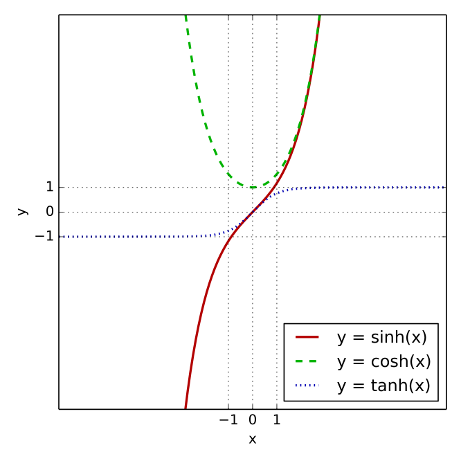
我们使用tanh作为隐藏状态的激活函数，其图像函数如下：

目标与计划

我们要从头实现一个RNN，执行一个情感分析任务——判断给定的文本是正面消息还是负面的。

这是我们要用的训练集：[data](rnn-from-scratch/data.py at master · vzhou842/rnn-from-scratch)

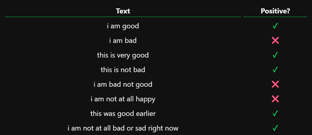
下面是一些训练集的样例：

由于这是一个分类问题，所以我们使用多对一的循环神经网络，即最终只使用最终的隐藏状态来生成一个输出。每个xi都是一个代表文本中一个单词的向量。输出y是一个二维向量，分别代表正面和负面。我们最终使用softmax将其转换为概率。

数据集预处理

神经网络无法直接识别单词，我们需要处理数据集，让它变成能被神经网络使用的数据格式。首先我们需要收集一下数据集中所有单词的词汇表：

vocab = list(set([w for text in train_data.keys() for w in text.split(" ")]))
vocab_size = len(vocab)

vocab是一个包含训练集中出现的所有的单词的列表。接下来，我们将为每一个词汇中的单词都分配一个整数索引，因为神经网络无法理解单词，所以我们要创造一个单词和整数索引的关系：

word_to_idx = {w:i for i,w in enumerate(vocab)}
idx_to_word = {i:w for i,w in enumerate(vocab)}

我们还要注意循环神经网络接收的每个输入都是一个向量xi，我们需要使用one-hot编码，将我们的每一个输入都转换成一个向量。对于一个one-hot向量，每个词汇对应于一个唯一的向量，这种向量出了一个位置外，其他位置都是0，在这里我们将每个one-hot向量中的1的位置，对应于单词的整数索引位置。

也就是说，我们的词汇表中有n个单词，我们的每个输入xi就应该是一个n维的one-hot向量。我们写一个函数，以用来创建向量输入，将其作为神经网络的输入：

def createInputs(text):
    inputs = []
    for w in text.split(" "):
        v = np.zeros((vocab_size,1))	# 创建一个vocab_size*1的全零向量
        v[word_to_idx[w]] = 1
        inputs.append(v)
    return inputs

向前传播

现在我们开始实现我们的RNN，我们先初始化我们所需的3个权重和2个偏置：

from numpy.random import randn	# 正态分布随机函数
class RNN:
    def __init__(self, input_size, output_size, hidden_size=64):
        # weights
        self.Whh = randn(hidden_size,hidden_size) / 1000
        self.Wxh = randn(hidden_size,input_size) / 1000
        self.Why = randn(output_size,hidden_size) / 1000
        # biases
        self.bh = np.zeros((hidden_size,1))
        self.by = np.zeros((output_size,1))

我们通过np.random.randn()从标准正态分布中初始化我们的权重。接下来我们将根据公式：

$$\begin{aligned} h_t &= tanh(W_{xh}x_t + W_{hh}h_{t-1}+b_h) \\ y_t &= W_{hy}h_t + b_y \end{aligned}$$

实现我们的向前传播函数:

    def forward(self,inputs):
        h = np.zeros((self.Whh.shape[0],1)) # 在刚开始我们的h是零向量，在此之前没有先前的h
        for i,x in enumerate(inputs):
            h = np.tanh(self.Wxh @ x + self.Whh @ h + self.bh) # @是numpy中的矩阵乘法符号
        y = self.Why @ y + self.by
        return y,h

现在我们的RNNs神经网络已经可以运行了：

from data import *
import numpy as np
from numpy.random import randn

def createInputs(text):
    inputs = []
    for w in text.split(" "):
        v = np.zeros((vocab_size,1))
        v[word_to_idx[w]] = 1
        inputs.append(v)
    return inputs

def softmax(x):
    return np.exp(x) / sum(np.exp(x))

class RNN:
    def __init__(self, input_size, output_size, hidden_size=64):
        # weights
        self.Whh = randn(hidden_size,hidden_size) / 1000
        self.Wxh = randn(hidden_size,input_size) / 1000
        self.Why = randn(output_size,hidden_size) / 1000
        # biases
        self.bh = np.zeros((hidden_size,1))
        self.by = np.zeros((output_size,1))

    def forward(self,inputs):
        h = np.zeros((self.Whh.shape[0],1))
        for i,x in enumerate(inputs):
            h = np.tanh(self.Wxh @ x + self.Whh @ h + self.bh)
        y = self.Why @ h + self.by
        return y,h

RNNs = RNN(vocab_size,2)
inputs = createInputs('i am very good')
out, h = RNNs.forward(inputs)
probs = softmax(out)
print(probs)
# [[0.50000228],[0.49999772]]

这里我们用到了softmax函数，softmax函数可以将任意的实值转换为概率（主要用于多分类任务）。它的核心作用是将网络的原始输出，转换为各类别的概率，使得所有概率之和为1。其公式如下

$$\begin{aligned} Softmax(z_i) = \frac{e^{z_i}}{\sum_{j=1}^{C}e^{z_j}} \end{aligned}$$

反向传播

为了训练我们RNNs，我们首先需要选择一个损失函数。对于分类模型，Softmax函数经常和交叉熵损失函数配合使用。它的计算方式如下：

$$\begin{aligned} L = -ln(p_c) \end{aligned}$$

其中pc是我们的RNNs对正确类别的预测概率（正面或负面）。例如，如果一个正面文本被我们的RNNs预测为90%的正面，那么可以计算出损失为：

$$\begin{aligned} L = -ln(0.90) = 0.105 \end{aligned}$$

既然有损失函数了，我们就可以使用梯度下降来训练我们的RNN以减小损失。

计算

首先从计算$\frac{\partial L}{\partial y}$开始，我们有：

$$\begin{aligned} L &= -ln(p_c) = -ln(softmax(y_c)) \\ \frac{\partial L}{\partial y} &= \frac{\partial L}{\partial p_c}* \frac{\partial p_c}{\partial y_i} \\ \frac{\partial L}{\partial p_c} &= -\frac{1}{p_c} \\ \frac{\partial p_c}{\partial y_i} &= \begin{cases} \frac{\partial p_i}{\partial y_i} = \frac{e^{y_i}\sum_{j}e^{y_j}-(e^{y_i})^2}{(\sum_{j}e^{y_j})^2} = p_i(1-p_i)&\text{if c=i} \\ \frac{\partial p_c}{\partial y_i} = \frac{e^{y_i}\sum_{j}e^{y_j}-(e^{y_i})^2}{(\sum_{j}e^{y_j})^2} = -p_cp_i&\text{if c!=i} \end{cases} \\ \frac{\partial L}{\partial y} &= \begin{cases} -\frac{1}{p_i} * p_i(1-p_i) = p_i-1 & \text{if c=i} \\ -\frac{1}{p_c} * (-p_cp_i) = p_i & \text{if c!=i} \end{cases} \end{aligned}$$

接下来我们尝试对Why和by的梯度，它们将最终隐藏状态转换为RNNs的输出。我们有：

$$\begin{aligned} \frac{\partial L}{\partial W_{hy}} &= \frac{\partial L}{\partial y} *\frac{\partial y}{\partial W_{hy}} \\ y &= W_{hy}h_n + b_y \\ \\ \frac{\partial y}{\partial W_{hy}} &= h_n \to \frac{\partial L}{\partial W_{hy}} = \frac{\partial L}{\partial y}h_n \\ \frac{\partial y}{\partial b_{y}} &= 1 \to \frac{\partial L}{\partial b_{y}} = \frac{\partial L}{\partial y} \end{aligned}$$

最后我们还需要Whh,Wxh和bh的梯度。由于梯度在每一步中都会被使用，所以根据时间展开和链式法则，我们有：

$$\begin{aligned} \frac{\partial L}{\partial W_{xh}} &= \frac{\partial L}{\partial y}\sum_{t=1}^{T}\frac{\partial y}{\partial h_t}*\frac{\partial h_t}{\partial W_{xh}} \\ \end{aligned}$$

这是因为L会被y所影响，而y被hT所影响，而hT又依赖于h(T-1)直到递归到h1，因此Wxh通过所有中间状态影响到L，所以在任意时间t，Wxh的贡献为：

$$\begin{aligned} \frac{\partial L}{\partial W_{xh}} \Big|_t &= \frac{\partial L}{\partial y}*\frac{\partial y}{\partial h_t}*\frac{\partial h_t}{\partial W_{xh}} \\ \end{aligned}$$

现在我们对其进行计算：

$$\begin{aligned} h_t &= tanh(W_{xh}x_t + W_{hh}h_{t-1}+b_h) \\ \frac{dtanh(x)}{dx} &= 1-tanh^2(x) \\ \\ \frac{\partial h_t}{\partial W_{xh}} &= (1-h_t^2)x_t \\ \frac{\partial h_t}{\partial W_{hh}} &= (1-h_t^2)h_{t-1} \\ \frac{\partial h_t}{\partial b_h} &= (1-h_t^2) \\ \end{aligned}$$

最后我们需要计算出$\frac{\partial y}{\partial h_t}$。我们可以递归的计算它： $$ \begin{aligned} \frac{\partial y}{\partial h_t} &= \frac{\partial y}{\partial h_{t+1}}*\frac{\partial h_{t+1}}{\partial h_t} \ &= \frac{\partial y}{\partial h_{t+1}}(1-h_t^2)W_{hh} \

\end{aligned} $$ 由于我们是反向训练的，$\frac{\partial y}{\partial h_{t+1}}$是已经计算的最后一步的梯度$\frac{\partial y}{\partial h_n}=W_{hh}$。至此为止我们的推导就结束了

实现

由于反向传播训练需要用到前向传播中的一些数据，所以我们将其进行存储：

    def forward(self,inputs):
        h = np.zeros((self.Whh.shape[0],1))
        # 数据存储
        self.last_inputs = inputs
        self.last_hs = {0:h}
        for i,x in enumerate(inputs):
            h = np.tanh(self.Wxh @ x + self.Whh @ h + self.bh)
            self.last_hs[i+1] = h   # 更新存储
        y = self.Why @ h + self.by
        return y,h

现在我们可以开始实现backprop()了：

    def backprop(self,d_y,learn_rate=2e-2):
        # d_y: 是损失函数对于输出的偏导数 d_L/d_y 的结果
        n = len(self.last_inputs)
        # 计算dL/dWhy,dL/dby
        d_Why = d_y @ self.last_hs[n].T
        d_by = d_y
        # 初始化dL/dWhh,dL/dWxh,dL/dbh为0
        d_Whh = np.zeros(self.Whh.shape)
        d_Wxh = np.zeros(self.Wxh.shape)
        d_bh = np.zeros(self.bh.shape)
        # 计算dL/dh
        d_h = self.Why.T @ d_y  # 因为dy/dh = Why 所以 dL/dh = Why * dL/dy

        # 随时间的反向传播
        for t in reversed(range(n)):
            # 通用数据 dL/dh * (1-h^2)
            temp = (d_h * (1 - self.last_hs[t+1] ** 2))
            # dL/db = dL/dh * (1-h^2)
            d_bh += temp
            # dL/dWhh = dL/dh * (1-h^2) * h_{t-1}
            d_Whh += temp @ self.last_hs[t].T
            # dL/dWxh = dL/dh * (1-h^2) * x
            d_Wxh += temp @ self.last_inputs[t].T
            # Next dL/dh = dL/dh * (1-h^2) * Whh
            d_h = self.Whh @ temp

        # 梯度剪裁(防止梯度过大导致梯度爆炸问题)
        for d in [d_Wxh,d_Whh,d_Why,d_by,d_bh]:
            np.clip(d,-1,1,out=d)

        # 梯度下降训练
        self.Whh -= learn_rate * d_Whh
        self.Wxh -= learn_rate * d_Wxh
        self.Why -= learn_rate * d_Why
        self.bh -= learn_rate * d_bh
        self.by -= learn_rate * d_by

由于这一部分的编写涉及到矩阵的变换，所以在编写时，一定要清楚每个变量的状态，以免造成数学错误。例如，以上程序中@的左乘右乘顺序不能随意改变。

训练

我们现在需要写一个接口，将我们的数据"喂"给神经网络，并量化损失和准确率，用于训练我们的神经网络。

def processData(data, backprop=True):
    # 打乱数据集 避免顺序偏差
    items = list(data.items())
    random.shuffle(items)

    loss = 0
    num_correct =0
    for x,y in items:
        inputs = createInputs(x)
        target = int(y)
        # 前向传播计算
        out,_ = RNN.forward(inputs)
        probs = softmax(out)
        # 计算损失与准确度
        loss -= np.log(probs[target])
        num_correct += int(np.argmax(probs) == target)

        if backprop:
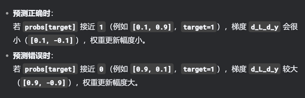
            d_L_d_y = probs
            d_L_d_y[target] -= 1
            RNN.backprop(d_L_d_y)
    
    return loss/len(data),num_correct /len(data)

这里对于$\frac{\partial L}{\partial y}$的初始化我们需要重点关注一下。由于我们使用的是，交叉熵损失+Softmax函数来进行处理。对于输出层，我们有一个简洁的表达式来进行处理:

$$\begin{aligned} \frac{\partial L}{\partial y} = probs - onehot(target) \end{aligned}$$

这里我选用AI的解释来直观的感受为什么这么做:

我们在前面也推导过这个原因

$$\begin{aligned} \frac{\partial L}{\partial y} &= \begin{cases} -\frac{1}{p_i} * p_i(1-p_i) = p_i-1 & \text{if c=i} \\ -\frac{1}{p_c} * (-p_cp_i) = p_i & \text{if c!=i} \end{cases} \end{aligned}$$

最后我们编写训练循环，来对我们的内容进行训练：

for epoch in range(1000):
    train_loss, train_acc = processData(train_data)

    if epoch % 100 == 99:
        print('--- Epoch %d' % (epoch + 1))
        print('Train:\tLoss %.3f | Accuracy: %.3f' % (train_loss, train_acc))

        test_loss, test_acc = processData(test_data, backprop=False)
        print('Test:\tLoss %.3f | Accuracy: %.3f' % (test_loss, test_acc))

执行可以看到完整的训练过程。

使用

既然完成了训练，那么我们可以尝试与其进行沟通，我们可以写一个接口用于和它进行对话：

def predict(probs, mid=0.5):
    positive_prob = probs[1]
    return "Yes,you are positive ^_^" if positive_prob > mid else "No,you are negative qwq"


print("please wait some time to train")

for epoch in range(1000):
    processData(train_data)

while True:
    text = input("please input a sentence: ").lower()
    inputs = createInputs(text)
    out, _ = rnn.forward(inputs)
    probs = softmax(out)
    print(predict(probs))

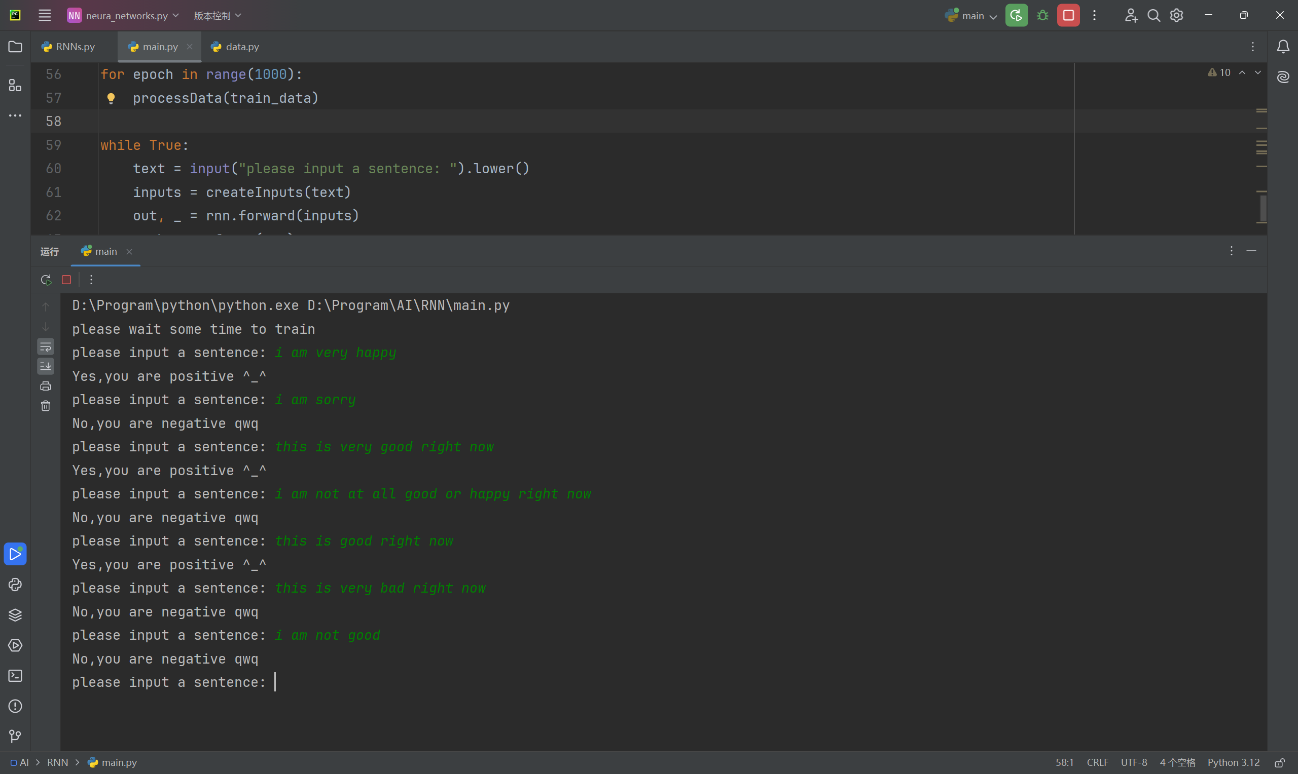
哈哈效果还可以，只不过只能检测到训练集中用过的单词。