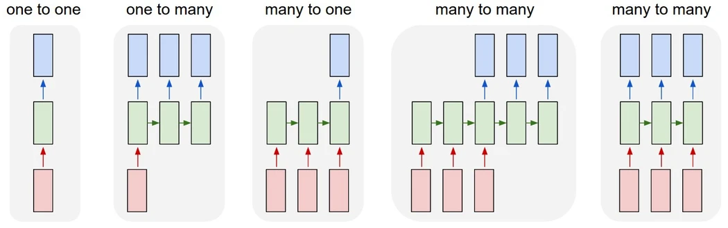
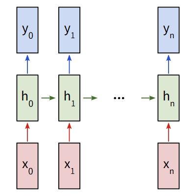
上一篇文章中我们学习了循环神经网络，我们现在已经基本理解了神经网络怎么去处理数据/序列。可是对于图片、音频、文件之类的数据，我们该怎么去处理呢？相较于数据、序列，对图片使用传统神经网络会导致更大的开销。其他的数据类型也是同理，所以接下来我们将要认识卷积神经网络。

卷积神经网络简介

卷积神经网络的一个经典应用场景是对图像进行分类，可是我们可不可以使用普通的神经网络来实现呢？可以，但是没必要。对于图像数据处理，我们需要面临两个问题：

• 图像数据很大 假如我们要处理的图像大小是100x100甚至更大。那么构建一个处理100x100的彩色图像的神经网络，我们需要100x100x3 = 30000个输入特征。我们用一个1024个节点的中间层，意味着我们在一层中就要训练30000x1024 = 30720000个权重。这样会导致我们的神经网络十分庞大
• 图像特征的位置会改变 同一个特征可能是在图像中的不同位置，你可能可以训练出一个对于特定图像表现良好的网络。但是当你对图像进行一定的偏移，可能就会导致结果发生错误的改变

使用传统的神经网络来解决图像问题，无异于是浪费的。它忽视了图像中任意像素与其邻近像素的上下文关系，图像中的物体是由小范围的局部特征组成的，对每个像素都进行分析，是毫无意义的。

所以我们需要使用卷积神经网络来解决这些问题。

目标

这一次我们的目标是实现一个手写数字识别的卷积神经网络，用到的是MNIST的手写数字数据集。也就是给定一个图像，将其分类为一个数字。

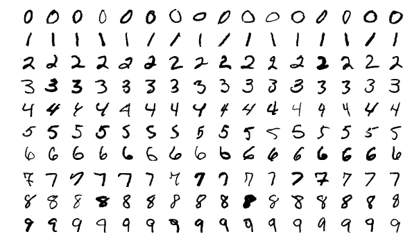
MNIST数据集中的每张图片都是28*28的大小，包含一个居中的灰度数字。我们将根据这个数据集来对神经网络进行训练。

卷积

我们首先要理解卷积神经网络中的卷积是什么意思。卷积实际上是一种加权平均的操作。它的相当于一个滤波器，能够提取原始数据中的某种特定特征。我们往往使用卷积核来进行这个操作。

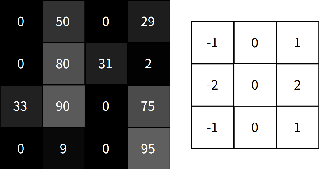
而神经网络中的卷积层则是根据过滤器实现对局部特征的处理，我们以下面这个操作为例：

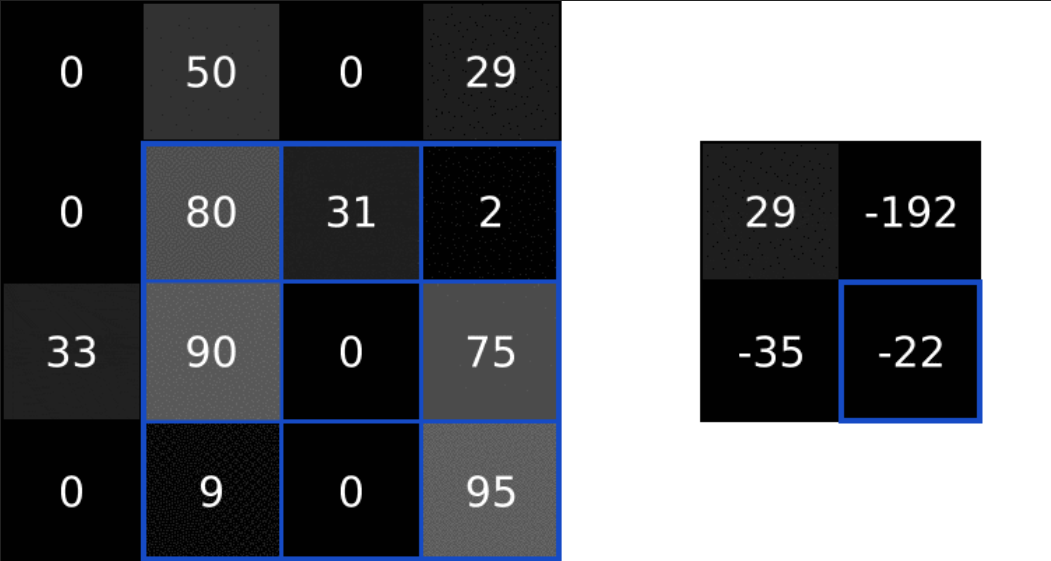
对于一个垂直特征的卷积核，我们可以计算出这里的特征值

我们们可以通过对图像中的数据进行卷积操作从而实现对局部特征的提取。这就和我们将要用到的卷积核有关了。

卷积核

这是一个垂直sobel滤波器，通过它对图像进行卷积操作，我们可以提取出图像的垂直特征：

同样的，我们有对应的水平SObel卷积核，可以提取出图像的水平特征：

而Sobel滤波器，我们可以理解成边缘检测器。通过提取手写数字边缘的特征，有利于网络在后续更好的进行图像识别。

填充

对于卷积这一步，我们对一个4x4的输入图像使用一个3x3的滤波器，我们会得到一个2x2的输出图像。如果我们希望输出图像和输入图像保持相同的大小。我们则需要向周围添加0，使得滤波器可以在更多的位置上覆盖

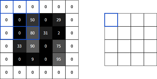
这种操作，我们称之为相同填充。如果不适用任何填充，我们称之为有效填充。

卷积层的使用

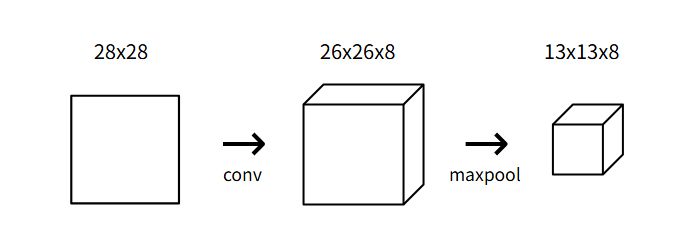
我们现在知道卷积层通过使用一组滤波器将输入图像转换为输出图像的卷积层了。我们将使用一个具有8个滤波器的小卷积层作为我们网络中的起始层，意味着，它将28x28的输入图像转换为26x26x8的输出体积：

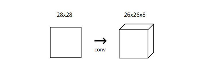
每个卷积层的8个过滤器产生一个26x26的输出，这是因为我们用到的是3x3的卷积核作为我们的滤波器，所以我们需要训练的权重有3x3x8 = 72个权重

实现

现在我们尝试用代码实现一个卷积层：

1
2
3
4
5
6
7
8

import numpy as np

class Conv3x3:
    # 使用3x3滤波器的卷积层
    def __init__(self,num_filters):
        self.num_filters = num_filters
        # 这里除以3是为了对权重进行初始化
        self.filters = np.random.randn(num_filters,3,3) / 9

我们注意到我们对生成的卷积核中做了一个权重初始化的工作，这是因为：

• 如果初始权重太大，那么输入数据经过卷积计算之后会变得很大，在反向传播的过程中梯度值也会变得很大，从而导致参数无法收敛，即梯度爆炸
• 如果初始权重太小，由于激活函数的作用，输入的数据会层层缩小，导致反向传播过程中的梯度值变得绩效。难以实现对权重的有效更新，我们称之为梯度消失

这里我们用到Xavier初始化来解决这个问题，他指出，在保持网络层在初始化时，其输入核和输出的方差应该尽可能的相同。这样信号就可以在网络中稳定的传播。

我们设输入为y输出为x，权重矩阵为W。则有： $$ \begin{align*} Var(W) = \frac{1}{n_{in}} \end{align*} $$ 其中n_in是输入的节点数量，这里就是3x3，所以初始化时需要/9

接下来是实际的卷积部分的实现：

1
2
3
4
5
6
7
8
9
10
11
12
13
14
15
16
17
18
19
20
21
22
23

class Conv3x3:
    # 使用3x3滤波器的卷积层
    def __init__(self,num_filters):
        self.num_filters = num_filters
        self.filters = np.random.randn(num_filters,3,3) / 9

    def iterate_regions(self,image):
        # 返回所有可以卷积的3x3的图像区域
        h,w = image.shape
        for i in range(h-2):
            for j in range(w-2):
                im_region = image[i:(i+3),j:(j+3)]
                yield im_region,i,j

    def forward(self,input):
        # 执行卷积层的前向传播 输出一个26x26x8的三维输出数组
        h,w = input.shape
        output = np.zeros((h-2,w-2,self.num_filters))
        for im_region,i,j in self.iterate_regions(input):
            # 这里用到的是numpy中隐藏的广播机制，详情参考numpy
            # 这里im_region*self.filters的大小是(8,3,3),求和是对行列求和,所以axis=(1,2)
            output[i,j] = np.sum(im_region * self.filters,axis=(1,2))
        return output

这里我们很多用法涉及到numpy的一些高级使用，可以在这里参考NumPy现在我们可以检查我们的卷积层是否输出了我们理想的结果:

1
2
3
4
5
6
7
8

from conv import Conv3x3
import tensorflow as tf		# 由于MNIST数据集URL地址有问题，所以这里使用keras库

(x_train, y_train), (x_test, y_test) = tf.keras.datasets.mnist.load_data()

conv = Conv3x3(8)
output = conv.forward(x_train[0])
print(output.shape)	# (26,26,8) 

池化

图像中的相邻元素往往是相似的，所以卷积层输出中，通常相邻元素产生相似的值。结果导致卷积层输出中包含了大量的冗余信息。为了解决这个问题我们需要对数据进行池化

它所做的事情很简单，往往是将输出中的值聚合称为更小的尺寸。池化往往是通过简单的操作，如max,min,average实现的。比如下面就是一个池化大小为2的最大池化操作

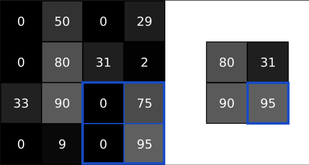
池化将输入的宽度和高度除以池化大小。在我们的卷积神经网络中，我们将在初始卷积层之后放置一个池化大小为2的最大池化层，池化层将26x26x8的输入转化为13x13x8的输出：

实现

我们现在用代码实现和conv类相似的MaxPool2类：

1
2
3
4
5
6
7
8
9
10
11
12
13
14
15
16
17
18
19

import numpy as np
class MaxPool2:
    # 池化尺寸为2的最大池化层
    def iterate_regions(self,image):
        h,w,_ = image.shape
        new_h = h // 2
        new_w = w // 2
        for i in range(new_h):
            for j in range(new_w):
                im_region = image[i*2:(i+1)*2,j*2:(j+1)*2]
                yield im_region,i,j
    
    def forward(self,input):
        h,w,num_filters = input.shape
        output = np.zeros((h//2,w//2,num_filters))        
        for im_region,i,j in self.iterate_regions(input):
            # 这里im_region的大小是(3,3,8)因此我们只需要对行列求最大，故axis=(0,1)
            output[i,j] = np.amax(im_region,axis=(0,1))            
        return output

这个类和之前实现的Conv3x3类类似，关键在于从一个给定的图像区域中找到最大值，我们使用数组的最大值方法np.amax()来实现。我们来测试一下池化层：

1
2
3
4
5
6
7
8
9
10
11
12

from conv import Conv3x3
from maxpool import MaxPool2
import tensorflow as tf

(x_train, y_train), (x_test, y_test) = tf.keras.datasets.mnist.load_data()

conv = Conv3x3(8)
pool = MaxPool2()

output = conv.forward(x_train[0])
output = pool.forward(output)
print(output.shape)	# (13,13,8)

Softmax层

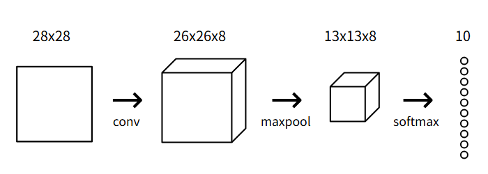
现在我们通过前两层，已经提取出了数字特征，现在我们希望能够赋予其实际预测的能力。对于多分类问题，我们通常使用Softmax层作为最终层——这是一个使用Softmax函数作为激活函数的全连接层（全连接层就是每个节点都与前一层的每个输入相联）

我们将使用一个包含10个节点的Softmax层作为CNN的最后一层，每个节点代表一个数字。层中的每个节点都连接到之前的输出中。在Softmax变化之后，概率最高的数字就是我们的输出。

交叉熵损失

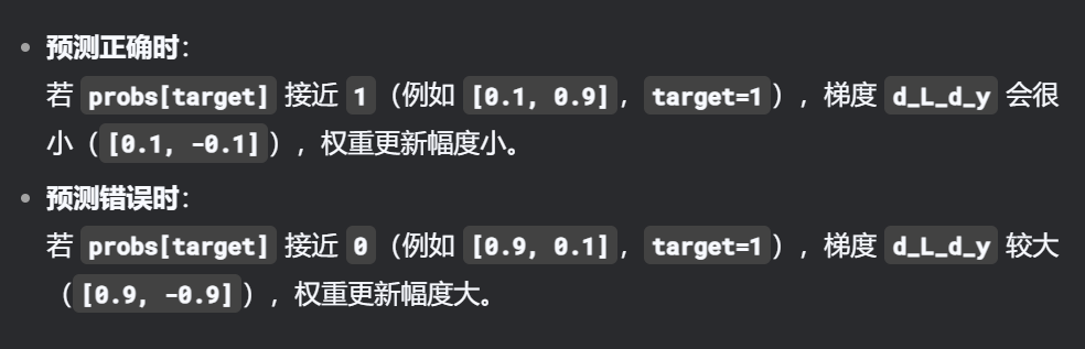
我们现在既然可以输出最终的预测结果了，它输出的结果是一个概率，用来量化神经网络的对其预测的信心。同样的，我们也需要一种方法来量化每次预测的损失。这里我们使用交叉熵损失来解决这个问题： $$ \begin{align*} L = -ln(p_c) \end{align*} $$ 其中c指的是正确的类别，即正确的数字。而p_c代表类别c的预测概率。我们希望损失越低越好，对网络的损失进行量化，有利于后续的神经网络训练。

实现

我们同上步骤，实现一个Softmax层类：

1
2
3
4
5
6
7
8
9
10
11
12
13

import numpy as np
class Softmax:
    # 全连接softmax激活层
    def __init__(self, input_len, nodes):
        self.weights = np.random.randn(input_len,nodes) / nodes
        self.biases = np.zeros(nodes)

    def forward(self, input):
        # 由于输入是一个输入体积,我们用flatten将其展平,变成一个一维的输出向量
        input = input.flatten()
        totals = np.dot(input,self.weights) + self.biases
        exp = np.exp(totals)
        return exp/np.sum(exp,axis=0)

现在，我们已经完成了CNN的整个前向传播，我们可以简单的测试一下：

1
2
3
4
5
6
7
8
9
10
11
12
13
14
15
16
17
18
19
20
21
22
23
24
25
26
27
28
29
30
31
32
33
34
35
36
37
38
39
40
41
42
43

import numpy as np

from conv import Conv3x3
from maxpool import MaxPool2
from softmax import Softmax
import tensorflow as tf

(x_train, y_train), (x_test, y_test) = tf.keras.datasets.mnist.load_data()

test_images = x_test[:1000]
test_labels = y_test[:1000]

conv = Conv3x3(8)
pool = MaxPool2()
softmax = Softmax(13*13*8,10)

def forward(image,label):
    out = conv.forward((image / 255) - 0.5)
    out = pool.forward(out)
    out = softmax.forward(out)

    loss = -np.log(out[label])
    acc = 1 if np.argmax(out) == label else 0

    return out,loss,acc


print("Start!")
loss = 0
num_correct = 0

for i,(im,label) in enumerate(zip(test_images,test_labels)):
    _, l, acc = forward(im,label)
    loss += l
    num_correct += acc

    if i%100 == 99:
        print(
            '[Step %d] Past 100 steps :Average Loss %.3f | Accuracy %d%%' %
            (i+1,loss/100,num_correct)
        )
        loss = 0
        num_correct = 0

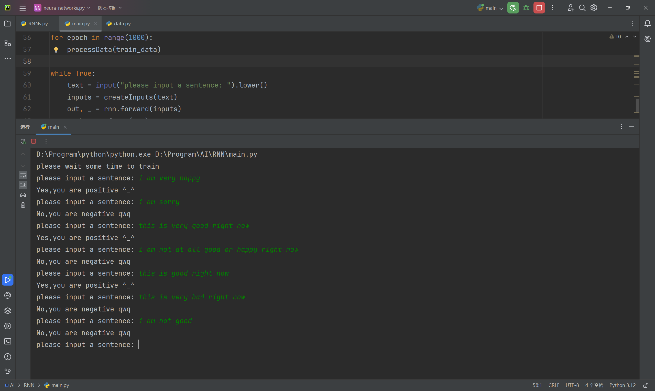
我们可以得到下面的输出：

1
2
3
4
5
6
7
8
9
10
11

Start!
[Step 100] Past 100 steps :Average Loss 2.566 | Accuracy 13%
[Step 200] Past 100 steps :Average Loss 2.447 | Accuracy 13%
[Step 300] Past 100 steps :Average Loss 2.500 | Accuracy 13%
[Step 400] Past 100 steps :Average Loss 2.520 | Accuracy 10%
[Step 500] Past 100 steps :Average Loss 2.431 | Accuracy 9%
[Step 600] Past 100 steps :Average Loss 2.477 | Accuracy 6%
[Step 700] Past 100 steps :Average Loss 2.491 | Accuracy 11%
[Step 800] Past 100 steps :Average Loss 2.598 | Accuracy 7%
[Step 900] Past 100 steps :Average Loss 2.545 | Accuracy 7%
[Step 1000] Past 100 steps :Average Loss 2.610 | Accuracy 10%

这是因为我们对权重进行了随机初始化，所以现在神经网络的表现更像是随机猜测，所以准确率趋近于10%

今天是8月24号，暑假已然过去了2/3，我打算明天就提前返校。我想对我的暑假做一个总结，这个暑假学了很多东西，相较于平时有更多的集中连续的时间可以用了学习，提升个人的能力。在校期间，我更多是用一些零散的时间来通过做项目来学习。但感觉难以长时间的专注在一个知识点上。始终是项目驱动学习，被动的去了解一些内容，暑假的话有大把的时间，可以去了解自己感兴趣的内容。我这个暑假主要学习了这些内容：

• 处理器 及其 流水线机制
• 程序性能优化简单了解
• 存储器层次结构的认识
• 简单算法入门 与 少量的刷题
• 链接编译过程
• 深度学习简单神经网络的构造 与 原理认识
• 异常控制流机制
• Linux shell编程 以及 简单指令的使用

这么一看学到的东西很多，但是大多数都是浅尝辄止，我打算多多接触之后再来明确自己感兴趣的方向。接下来是对我暑假的批评和反思。从7.3暑假开始到8.24今天，一共是52天，自由可支配（除去睡觉吃饭休息）的时间大概有600+个小时，我每次的学习时长可能也就4~5个小时，零零散散学了25天左右。剩下的时间浪费在打游戏，看动漫，看电影，看小说上面。

我暑假前定了很多目标，基本一个都没达到，超级灰心。但是，这也是意料之中的事情，取乎其上、得乎其中。所以我打算早点返校，好好用这最后的几天拯救一下我的暑假。但是怎么评价这个暑假呢，一直以来我都对自己有着很高的期望，但是通过这个暑假，我很好的认识清楚了自己的懒惰性，我也不太喜欢这样，但是自控力还是太差了，我也会好好的反思自己的行为。其次是这个暑假开拓了很多眼界，我意识到了和别人的差距，我总是把目光拘于学校，年级，班级，寝室，甚至是自己。我在网上看到了，认识到了很多优秀的人，感受到了差距，所以我打算继续前行，去学习各种感兴趣的内容。

对于下个学期的，我也是略有想法。下个学期课程十分繁重，但是大多是专业课程。这个是我的优势，专业课程内容我有很好的基础，我打算不跟着学校的计划走，我打算跟着南京大学的课程设计进行学习，计组方面打算跟着它们的PA学习，操作系统打算跟着JYY老师的课程深入了解一下。数据结构与算法，我打算制定一个刷题计划，要保证每天有一定的算法学习时间。还有科研方面，我打算联系LLF老师尝试写出我的第一篇论文。暑假我看着两位学长保研，我一直以为保研就是对绩点要求很高，但是实际上本科期间的科研成果是及其重要的，我这个暑假一直疏于对这方面的学习。下个学期，我打算花大部分的时间在这上面。

总结下来，下个学期的几个主要任务：

• 利用专业知识的优势，提升绩点成绩，加深对专业知识的掌握理解
• 提高算法能力，争取在下一学年中能够掌握常见的算法题型
• 深入学习逆向工程和二进制漏洞审计的，多刷题，强化竞赛能力
• 掌握最基本的科研能力，要开始入手自己的第一篇论文
• 学习计算机网络，完善技术栈

不过我还是很期待9月份的到来，一个是9.3有大阅兵，我特别想看。还有一个是丝之歌发售，我特别想玩，我打算一出就开始玩，通宵玩，累了就睡，饿了就吃，醒了就玩。我初步估计可能通关需要20~30小时，也就是[9.3,9.6]好好玩四天。剩下的时间就对暑期的计划做一个收尾。

在上一篇博客中，我们完成了一个简单的前馈神经网络，完成了对根据身高体重对性别进行猜测的神经网络，以及对他的训练。但是我们不该止步于此，接下来我们将尝试编写一个RNN循环神经网络，并认识它背后的原理。

循环神经网络简介

循环神经网络是一种专门用于处理序列的神经网络，因此其对于处理文本方面十分有效。且对于前馈神经网络和卷积神经网络，我们发现：它们都只能处理预定义的尺寸——接受固定大小的输入并产生固定大小的输出。但是循环神经网络可以处理任意长度的序列，并返回。它可以是这样的：

这种处理序列的方式可以实现很多功能。例如，文本翻译，事件评价… 我们的目标是让它完成对一个评论的判断（是正面的还是负面的）。将待分析的文本输入神经网络然后，然后给出判断。

实现方式

我们考虑一个输入为x0,x1,x2,...,xn，输出为y0,y1,y2,..,yn的多对多循环神经网络。这些xi和yi是向量，可以是任意维度。RNNs通过迭代更新一个隐藏状态h，重复这些步骤：

• 下一个隐藏状态h_t是前一个状态h_t-1和下一个输入x_t计算得出的
• 输出y_t是由当前的隐藏状态h_t计算得出的

这就是RNNs为什么是循环神经网络的原因，对于上面步骤的每一步中，都使用的是同一个权重。对于一个典型的RNNs，我们只需要使用3组权重就可以计算：

• W_xh 用于所有x_t -> h_t的连接
• W_hh 用于所有h_t-1 -> h_t的连接
• W_hy 用于所有h_t -> y_t的连接

同时我们还需要为两次输出设置偏置：

• b_h 计算h_t时的偏置
• b_y 计算y_t时的偏置

我们将权重表示为矩阵，将偏置表示为向量，从而组合成整个RNNs。我们的输出是： $$ \begin{align*} h_t &= tanh(W_{xh}x_t + W_{hh}h_{t-1}+b_h) \\ y_t &= W_{hy}h_t + b_y \end{align*} $$ 我们使用tanh作为隐藏状态的激活函数，其图像函数如下：

目标与计划

我们要从头实现一个RNN，执行一个情感分析任务——判断给定的文本是正面消息还是负面的。

这是我们要用的训练集：data

下面是一些训练集的样例：

由于这是一个分类问题，所以我们使用多对一的循环神经网络，即最终只使用最终的隐藏状态来生成一个输出。每个xi都是一个代表文本中一个单词的向量。输出y是一个二维向量，分别代表正面和负面。我们最终使用softmax将其转换为概率。

数据集预处理

神经网络无法直接识别单词，我们需要处理数据集，让它变成能被神经网络使用的数据格式。首先我们需要收集一下数据集中所有单词的词汇表：

1
2

vocab = list(set([w for text in train_data.keys() for w in text.split(" ")]))
vocab_size = len(vocab)

vocab是一个包含训练集中出现的所有的单词的列表。接下来，我们将为每一个词汇中的单词都分配一个整数索引，因为神经网络无法理解单词，所以我们要创造一个单词和整数索引的关系：

1
2

word_to_idx = {w:i for i,w in enumerate(vocab)}
idx_to_word = {i:w for i,w in enumerate(vocab)}

我们还要注意循环神经网络接收的每个输入都是一个向量xi，我们需要使用one-hot编码，将我们的每一个输入都转换成一个向量。对于一个one-hot向量，每个词汇对应于一个唯一的向量，这种向量出了一个位置外，其他位置都是0，在这里我们将每个one-hot向量中的1的位置，对应于单词的整数索引位置。

也就是说，我们的词汇表中有n个单词，我们的每个输入xi就应该是一个n维的one-hot向量。我们写一个函数，以用来创建向量输入，将其作为神经网络的输入：

1
2
3
4
5
6
7

def createInputs(text):
    inputs = []
    for w in text.split(" "):
        v = np.zeros((vocab_size,1))	# 创建一个vocab_size*1的全零向量
        v[word_to_idx[w]] = 1
        inputs.append(v)
    return inputs

向前传播

现在我们开始实现我们的RNN，我们先初始化我们所需的3个权重和2个偏置：

1
2
3
4
5
6
7
8
9
10

from numpy.random import randn	# 正态分布随机函数
class RNN:
    def __init__(self, input_size, output_size, hidden_size=64):
        # weights
        self.Whh = randn(hidden_size,hidden_size) / 1000
        self.Wxh = randn(hidden_size,input_size) / 1000
        self.Why = randn(output_size,hidden_size) / 1000
        # biases
        self.bh = np.zeros((hidden_size,1))
        self.by = np.zeros((output_size,1))

我们通过np.random.randn()从标准正态分布中初始化我们的权重。接下来我们将根据公式： $$ \begin{align*} h_t &= tanh(W_{xh}x_t + W_{hh}h_{t-1}+b_h) \\ y_t &= W_{hy}h_t + b_y \end{align*} $$ 实现我们的向前传播函数:

1
2
3
4
5
6

def forward(self,inputs):
    h = np.zeros((self.Whh.shape[0],1)) # 在刚开始我们的h是零向量，在此之前没有先前的h
    for i,x in enumerate(inputs):
        h = np.tanh(self.Wxh @ x + self.Whh @ h + self.bh) # @是numpy中的矩阵乘法符号
    y = self.Why @ y + self.by
    return y,h

现在我们的RNNs神经网络已经可以运行了：

1
2
3
4
5
6
7
8
9
10
11
12
13
14
15
16
17
18
19
20
21
22
23
24
25
26
27
28
29
30
31
32
33
34
35
36
37
38

from data import *
import numpy as np
from numpy.random import randn

def createInputs(text):
    inputs = []
    for w in text.split(" "):
        v = np.zeros((vocab_size,1))
        v[word_to_idx[w]] = 1
        inputs.append(v)
    return inputs

def softmax(x):
    return np.exp(x) / sum(np.exp(x))

class RNN:
    def __init__(self, input_size, output_size, hidden_size=64):
        # weights
        self.Whh = randn(hidden_size,hidden_size) / 1000
        self.Wxh = randn(hidden_size,input_size) / 1000
        self.Why = randn(output_size,hidden_size) / 1000
        # biases
        self.bh = np.zeros((hidden_size,1))
        self.by = np.zeros((output_size,1))

    def forward(self,inputs):
        h = np.zeros((self.Whh.shape[0],1))
        for i,x in enumerate(inputs):
            h = np.tanh(self.Wxh @ x + self.Whh @ h + self.bh)
        y = self.Why @ h + self.by
        return y,h

RNNs = RNN(vocab_size,2)
inputs = createInputs('i am very good')
out, h = RNNs.forward(inputs)
probs = softmax(out)
print(probs)
# [[0.50000228],[0.49999772]]

这里我们用到了softmax函数，softmax函数可以将任意的实值转换为概率（主要用于多分类任务）。它的核心作用是将网络的原始输出，转换为各类别的概率，使得所有概率之和为1。其公式如下 $$ \begin{align*} Softmax(z_i) = \frac{e^{z_i}}{\sum_{j=1}^{C}e^{z_j}} \end{align*} $$

反向传播

为了训练我们RNNs，我们首先需要选择一个损失函数。对于分类模型，Softmax函数经常和交叉熵损失函数配合使用。它的计算方式如下： $$ \begin{align*} L = -ln(p_c) \end{align*} $$ 其中pc是我们的RNNs对正确类别的预测概率（正面或负面）。例如，如果一个正面文本被我们的RNNs预测为90%的正面，那么可以计算出损失为： $$ \begin{align*} L = -ln(0.90) = 0.105 \end{align*} $$

既然有损失函数了，我们就可以使用梯度下降来训练我们的RNN以减小损失。

计算

首先从计算$\frac{\partial L}{\partial y}$开始，我们有： $$ \begin{align*} L &= -ln(p_c) = -ln(softmax(y_c)) \\ \frac{\partial L}{\partial y} &= \frac{\partial L}{\partial p_c}* \frac{\partial p_c}{\partial y_i} \\ \frac{\partial L}{\partial p_c} &= -\frac{1}{p_c} \\ \frac{\partial p_c}{\partial y_i} &= \begin{cases} \frac{\partial p_i}{\partial y_i} = \frac{e^{y_i}\sum_{j}e^{y_j}-(e^{y_i})^2}{(\sum_{j}e^{y_j})^2} = p_i(1-p_i)&\text{if c=i} \\ \frac{\partial p_c}{\partial y_i} = \frac{e^{y_i}\sum_{j}e^{y_j}-(e^{y_i})^2}{(\sum_{j}e^{y_j})^2} = -p_cp_i&\text{if c!=i} \end{cases} \\ \frac{\partial L}{\partial y} &= \begin{cases} -\frac{1}{p_i} * p_i(1-p_i) = p_i-1 & \text{if c=i} \\ -\frac{1}{p_c} * (-p_cp_i) = p_i & \text{if c!=i} \end{cases} \end{align*} $$ 接下来我们尝试对Why和by的梯度，它们将最终隐藏状态转换为RNNs的输出。我们有： $$ \begin{align*} \frac{\partial L}{\partial W_{hy}} &= \frac{\partial L}{\partial y} *\frac{\partial y}{\partial W_{hy}} \\ y &= W_{hy}h_n + b_y \\ \\ \frac{\partial y}{\partial W_{hy}} &= h_n \to \frac{\partial L}{\partial W_{hy}} = \frac{\partial L}{\partial y}h_n \\ \frac{\partial y}{\partial b_{y}} &= 1 \to \frac{\partial L}{\partial b_{y}} = \frac{\partial L}{\partial y} \end{align*} $$ 最后我们还需要Whh,Wxh和bh的梯度。由于梯度在每一步中都会被使用，所以根据时间展开和链式法则，我们有： $$ \begin{align*} \frac{\partial L}{\partial W_{xh}} &= \frac{\partial L}{\partial y}\sum_{t=1}^{T}\frac{\partial y}{\partial h_t}*\frac{\partial h_t}{\partial W_{xh}} \\ \end{align*} $$ 这是因为L会被y所影响，而y被hT所影响，而hT又依赖于h(T-1)直到递归到h1，因此Wxh通过所有中间状态影响到L，所以在任意时间t，Wxh的贡献为： $$ \begin{align*} \frac{\partial L}{\partial W_{xh}} \Big|_t &= \frac{\partial L}{\partial y}*\frac{\partial y}{\partial h_t}*\frac{\partial h_t}{\partial W_{xh}} \\ \end{align*} $$ 现在我们对其进行计算： $$ \begin{align*} h_t &= tanh(W_{xh}x_t + W_{hh}h_{t-1}+b_h) \\ \frac{dtanh(x)}{dx} &= 1-tanh^2(x) \\ \\ \frac{\partial h_t}{\partial W_{xh}} &= (1-h_t^2)x_t \\ \frac{\partial h_t}{\partial W_{hh}} &= (1-h_t^2)h_{t-1} \\ \frac{\partial h_t}{\partial b_h} &= (1-h_t^2) \\ \end{align*} $$ 最后我们需要计算出$\frac{\partial y}{\partial h_t}$。我们可以递归的计算它： $$ $$ 由于我们是反向训练的，$\frac{\partial y}{\partial h_{t+1}}$是已经计算的最后一步的梯度$\frac{\partial y}{\partial h_n}=W_{hh}$。至此为止我们的推导就结束了

实现

由于反向传播训练需要用到前向传播中的一些数据，所以我们将其进行存储：

1
2
3
4
5
6
7
8
9
10

def forward(self,inputs):
    h = np.zeros((self.Whh.shape[0],1))
    # 数据存储
    self.last_inputs = inputs
    self.last_hs = {0:h}
    for i,x in enumerate(inputs):
        h = np.tanh(self.Wxh @ x + self.Whh @ h + self.bh)
        self.last_hs[i+1] = h   # 更新存储
    y = self.Why @ h + self.by
    return y,h

现在我们可以开始实现backprop()了：

1
2
3
4
5
6
7
8
9
10
11
12
13
14
15
16
17
18
19
20
21
22
23
24
25
26
27
28
29
30
31
32
33
34
35
36

def backprop(self,d_y,learn_rate=2e-2):
    # d_y: 是损失函数对于输出的偏导数 d_L/d_y 的结果
    n = len(self.last_inputs)
    # 计算dL/dWhy,dL/dby
    d_Why = d_y @ self.last_hs[n].T
    d_by = d_y
    # 初始化dL/dWhh,dL/dWxh,dL/dbh为0
    d_Whh = np.zeros(self.Whh.shape)
    d_Wxh = np.zeros(self.Wxh.shape)
    d_bh = np.zeros(self.bh.shape)
    # 计算dL/dh
    d_h = self.Why.T @ d_y  # 因为dy/dh = Why 所以 dL/dh = Why * dL/dy

    # 随时间的反向传播
    for t in reversed(range(n)):
        # 通用数据 dL/dh * (1-h^2)
        temp = (d_h * (1 - self.last_hs[t+1] ** 2))
        # dL/db = dL/dh * (1-h^2)
        d_bh += temp
        # dL/dWhh = dL/dh * (1-h^2) * h_{t-1}
        d_Whh += temp @ self.last_hs[t].T
        # dL/dWxh = dL/dh * (1-h^2) * x
        d_Wxh += temp @ self.last_inputs[t].T
        # Next dL/dh = dL/dh * (1-h^2) * Whh
        d_h = self.Whh @ temp

    # 梯度剪裁(防止梯度过大导致梯度爆炸问题)
    for d in [d_Wxh,d_Whh,d_Why,d_by,d_bh]:
        np.clip(d,-1,1,out=d)

    # 梯度下降训练
    self.Whh -= learn_rate * d_Whh
    self.Wxh -= learn_rate * d_Wxh
    self.Why -= learn_rate * d_Why
    self.bh -= learn_rate * d_bh
    self.by -= learn_rate * d_by

由于这一部分的编写涉及到矩阵的变换，所以在编写时，一定要清楚每个变量的状态，以免造成数学错误。例如，以上程序中@的左乘右乘顺序不能随意改变。

训练

我们现在需要写一个接口，将我们的数据”喂”给神经网络，并量化损失和准确率，用于训练我们的神经网络。

1
2
3
4
5
6
7
8
9
10
11
12
13
14
15
16
17
18
19
20
21
22
23

def processData(data, backprop=True):
    # 打乱数据集 避免顺序偏差
    items = list(data.items())
    random.shuffle(items)

    loss = 0
    num_correct =0
    for x,y in items:
        inputs = createInputs(x)
        target = int(y)
        # 前向传播计算
        out,_ = RNN.forward(inputs)
        probs = softmax(out)
        # 计算损失与准确度
        loss -= np.log(probs[target])
        num_correct += int(np.argmax(probs) == target)

        if backprop:
            d_L_d_y = probs
            d_L_d_y[target] -= 1
            RNN.backprop(d_L_d_y)
    
    return loss/len(data),num_correct /len(data)

这里对于$\frac{\partial L}{\partial y}$的初始化我们需要重点关注一下。由于我们使用的是，交叉熵损失+Softmax函数来进行处理。对于输出层，我们有一个简洁的表达式来进行处理: $$ \begin{align*} \frac{\partial L}{\partial y} = probs - onehot(target) \end{align*} $$ 这里我选用AI的解释来直观的感受为什么这么做:

我们在前面也推导过这个原因 $$ \begin{align*} \frac{\partial L}{\partial y} &= \begin{cases} -\frac{1}{p_i} * p_i(1-p_i) = p_i-1 & \text{if c=i} \\ -\frac{1}{p_c} * (-p_cp_i) = p_i & \text{if c!=i} \end{cases} \end{align*} $$ 最后我们编写训练循环，来对我们的内容进行训练：

1
2
3
4
5
6
7
8
9

for epoch in range(1000):
    train_loss, train_acc = processData(train_data)

    if epoch % 100 == 99:
        print('--- Epoch %d' % (epoch + 1))
        print('Train:\tLoss %.3f | Accuracy: %.3f' % (train_loss, train_acc))

        test_loss, test_acc = processData(test_data, backprop=False)
        print('Test:\tLoss %.3f | Accuracy: %.3f' % (test_loss, test_acc))

执行可以看到完整的训练过程。

使用

既然完成了训练，那么我们可以尝试与其进行沟通，我们可以写一个接口用于和它进行对话：

1
2
3
4
5
6
7
8
9
10
11
12
13
14
15
16

def predict(probs, mid=0.5):
    positive_prob = probs[1]
    return "Yes,you are positive ^_^" if positive_prob > mid else "No,you are negative qwq"


print("please wait some time to train")

for epoch in range(1000):
    processData(train_data)

while True:
    text = input("please input a sentence: ").lower()
    inputs = createInputs(text)
    out, _ = rnn.forward(inputs)
    probs = softmax(out)
    print(predict(probs))

哈哈效果还可以，只不过只能检测到训练集中用过的单词。

在网上冲浪的时候我们经常会看到一些点开与不点开会呈现不同结果的图片，我们称这种图片为”幻影坦克图”。因为它利用到了光学欺骗的原理，与红警中的幻影坦克相似，故得其名。今天，尝试了解下背后的原理，并自己动手实现一下这个功能。

原理

由于幻影坦克图需要涉及到alpha混合，所以我们使用的图像格式必须带有alpha通道。所以我们的首选就是png图像格式，我们将利用它的透明度来实现。最为核心的部分就是alpha通道作用于图片的计算公式： $$ \begin{align*} Color_{合} = Color_{前}*Alpha + Color_{后}*(1-Alpha) \end{align*} $$ 其中Color_合是混合后所被看到的颜色，Color_前是前景色，Color_后是背景色

我们可以通过改变背景色从而得到图像在背景上呈现的颜色，为了更好的背景效果，我们选择黑底与白底，分别是：(r_w,g_w,b_w,a_w) = (1,1,1,1)和(r_b,g_b,b_b,a_b) = (0,0,0,1)。现在我们可以计算出指定的带有透明度的图片分别在白底(r1,g1,b1)和黑底(r2,g2,b2)上呈现的颜色: $$ \begin{cases} r_1 = r*\alpha + (1-\alpha) \\ g_1 = g*\alpha + (1-\alpha) \\ b_1 = b*\alpha + (1-\alpha) \\ \\ r_2 = r*\alpha \\ g_2 = g*\alpha \\ b_2 = b*\alpha \end{cases} $$ 但是实际上我们想要把两张图片做成幻影坦克图，我们的(r1,g1,b1,1)和(r2,g2,b2,1)都应该是已知的，实际上我们要求解的应该是幻影坦克图(r,g,b,a)，所以我们调整方程组可得： $$ \begin{cases} \alpha = 1-r_1+r_2 \\ \alpha = 1-g_1+g_2 \\ \alpha = 1-b_1+b_2 \\ \\ r = \frac{r_2}{\alpha} = \frac{r_2}{1-r_1+r_2} \\ g = \frac{g_2}{1-g_1+g_2} \\ b = \frac{b_2}{1-b_1+b_2} \end{cases} $$ 现在我们发现透明度有三种不同的计算方式，此时我们该如何处理呢？在正常情况下，我们难以满足这三个式子相等。但是在灰度图下可以做到r = g = b，此时灰度图的亮度信息由像素亮度决定。同样的我们也需要注意到0 <= a <= 1的大小关系，因此我们必须有r1 >= r2。为了避免像素值也超出值域，我们在实现时，需要将r1压缩到[128,255]，将r2压缩到[0,127]

现在我们可以计算出我们想要的幻影坦克图片的每一个像素信息了。

代码实现

1
2
3
4
5
6
7
8
9
10
11
12
13
14
15
16
17
18
19
20
21
22
23
24
25
26
27
28
29

from PIL import Image
import numpy as np

def mix(img1, img2, output):
    # 灰度图转化RGB图
    img1 = Image.open(img1).convert("L").convert("RGB")
    img2 = Image.open(img2).convert("L").convert("RGB")
    # 调整图像大小
    img2 = img2.resize(img1.size)
    # 归一化
    imgarr1 = np.array(img1,dtype=np.float32) / 255.0
    imgarr2 = np.array(img2,dtype=np.float32) / 255.0
    # 压制像素 r1>= r2
    imgarr1 = 0.5 + 0.5 * imgarr1
    imgarr2 = 0.5 * imgarr2
    # 透明度计算
    alpha = 1 - imgarr1 + imgarr2
    alpha = np.clip(alpha,0,1)
    # 计算幻影坦克图颜色值
    rgb = imgarr2 / (alpha + 1e-6)
    rgb = np.clip(rgb,0,1)
    # 合并RGB与Alpha
    rgba = np.dstack((rgb,alpha.mean(axis=2)))
    # 输出图片
    img = Image.fromarray((rgba * 255).astype(np.uint8),"RGBA")
    img.save(output)

mix("D:/Photo/111.png","D:/Photo/123.png","D:/Micro/test.png")

我们可以看到以下效果：

优化

我们通过将图片转换成灰度图的形式从而实现了幻影坦克图，但是我们却丢失了RGB通道的颜色。有没有什么方式能够尽可能的保留原来的色彩信息呢？

我们回到这个公式： $$ \begin{cases} \alpha = 1-r_1+r_2 \\ \alpha = 1-g_1+g_2 \\ \alpha = 1-b_1+b_2 \\ \\ r = \frac{r_2}{\alpha} = \frac{r_2}{1-r_1+r_2} \\ g = \frac{g_2}{1-g_1+g_2} \\ b = \frac{b_2}{1-b_1+b_2} \end{cases} $$ 由于在RGBA模式下，一个像素只能有一个alpha通道，也就是说三个色彩通道只能使用一个alpha。所以我们怎么才能让$1-r_1+r_2-g_1+g_2-b_1+b_2rg b $呢？

我们可以通过两种方式来实现：

• 调整图片整体亮度

  我们知道，图像的亮度调整通常是通过线性放缩实现的： $$ \begin{align*} RGB_{new} = RGB_{original} * k\space(0<k<1) \end{align*} $$ 所以RGB值之间的差值也是随着线性放缩变化的。当我们的亮度趋近于0时，r ≈ g ≈ b是成立的，我们可以通过减少亮度，从而提升幻影坦克图的视觉效果。

• 设置插值平衡色彩与灰度的混合比例

  我们可以通过设置差值，来平衡色彩和灰度的混合比例，使得透明度的计算结果在RGB三个通道上趋于一致，，我们基于这个公式可以求出合适的插值： $$ \begin{align*} r_{new} &= r*lerp + gray*(1-lerp) \\ gray &= 0.299*r + 0.587*g + 0.114*b \end{align*} $$ 通过这种方式我们可以强制对齐alpha通道，并减少通道差异。

所以接下来，我们需要考虑合适的合适的亮度与色彩插值，以实现更好的效果。

对于亮度，我们有

由于人的眼睛对光的线性变化的感受是非线性的，所以即使我们把黑底图的亮度系数调暗到0.22，视觉上也只会认为颜色变暗了0.5。所以[0.18,0.22]是我们选取亮度最合适的区间。

对于色彩插值参数，参数越大，灰度平衡的比例就越小，图片能更好的保留色彩。我们希望白底图能够保留较多的色彩，且黑底图能够更加隐蔽，所以我们设置：

• 表图 lerp = [0.6,0.8]
• 里图 lerp = [0.2,0.4]

综上所述我们可以实现我们最终的效果了

最终实现

1
2
3
4
5
6
7
8
9
10
11
12
13
14
15
16
17
18
19
20
21
22
23
24
25
26
27
28
29
30
31
32
33
34
35
36
37
38
39
40
41
42
43
44
45
46
47
48
49
50
51
52
53
54
55
56
57
58

from PIL import Image,ImageEnhance
import numpy as np

class Phantom:
    def __init__(self):
        self.default = {
            'brightnessW': 1,
            'brightnessB': 0.8,
            'lerpW':0.8,
            'lerpB':0.8
        }

    def loadImage(self,img1,img2):	# 加载图片
        img1 = Image.open(img1).convert("RGB")
        img2 = Image.open(img2).convert("RGB")
        img2 = img2.resize(img1.size)
        return img1,img2

    def adjustBrightnedd(self,img,brightness):	# 亮度调节
        if brightness == 1:
            return img
        return ImageEnhance.Brightness(img).enhance(brightness)

    def blendColor(self,arr,lerp):	# 色彩插值平衡
        if lerp == 1.0:
            return arr
        gray = np.dot(arr,[0.299,0.587,0.114])
        return arr * lerp + gray[...,None] * (1-lerp)

    def generate(self,img1,img2,outpath,**kwargs):	
        params = {**self.default,**kwargs}
        # 加载图片
        img1, img2 = self.loadImage(img1,img2)
        # 亮度调整
        img1 = self.adjustBrightnedd(img1,params['brightnessW'])
        img2 = self.adjustBrightnedd(img2,params['brightnessB'])
        # 归一化
        arr1 = np.array(img1, dtype=np.float32) / 255.0
        arr2 = np.array(img2, dtype=np.float32) / 255.0
        # 压制像素 值域区分
        arr1 = 0.5 + 0.5 * arr1
        arr2 = 0.5 * arr2
        # 色彩差值平衡
        arr1 = self.blendColor(arr1,params['lerpW'])
        arr2 = self.blendColor(arr2,params['lerpB'])
        # 透明度计算
        alpha = np.clip(1-arr1+arr2,0,1)
        # 幻影坦克图像素计算
        rgb = np.clip(arr2/(alpha + 1e-6),0,1)
        rgba = np.dstack((rgb, alpha.mean(axis=2)))
        # 转化图片
        img = Image.fromarray((rgba * 255).astype(np.uint8), "RGBA")
        img.save(outpath)


if __name__ == '__main__':
    ph = Phantom()
    ph.generate("D:/Photo/q.jpg","D:/Photo/w.jpg","D:/Micro/test.png")

效果挺好滴，展示一下：

信号

我们已经认识到了操作系统怎么通过异常使得进程上下文切换，以实现异常控制流的实现。现在我们将尝试另一种实现——Linux信号，来允许进程和内核中断其他的进程。

我们可以将信号理解成一条消息，它通知进程系统中发生了某一个事件。每种信号类型都会对应于某种系统事件。然后由不同的处理程序去处理这个事件。我们可以通过man 7 signal来进一步的认识这些信号：

信号术语

传送一个信号到目的进程可以分作两个步骤：

• 发送信号：内核通过更新目的进程的上下文中的某个状态，从而实现发送一个信号给目的进程。发送信号一般有以下两种原因：1)内核检测到了一个系统事件，2)一个进程调用了kill函数，显式的要求内核发送一个信号给目的进程
• 接收信号：当目的进程被内核强迫对信号的发送做出反应时，我们就说它接受了信号。目的进程可以忽略这个信号，终止，或者通过执行信号处理程序的用户层来捕获这个信号。

一个发出但没有被接收的信号我们称之为待处理信号。在任何时刻一个类型只会有一个待处理信号。如果一个进程中有一个类型为k的待处理信号。接下来任何发送到这个进程的类型为k的信号都不会再排队等候，而是被丢弃。同时一个进程可以选择阻塞接受某种信号。如果一个信号被阻塞，它可以发送，但是不会再被接收，直到取消对它的阻塞。

这个实现通过内核为每个进程维护这一个信号处理集合实现。在pending向量中维护着一个待处理信号的集合，在blocked向量中维护着一个阻塞信号的集合。当一个信号类型为k的信号被发送时，目的进程会检查其pending位是否已被设置，若是则丢弃；不是则设置。然后检查其block位是否被阻塞，若是则丢弃；若不是则接受信号，并清除pending位。

发送信号

发送信号的机制，是基于进程组实现的。我们接下来进一步的理解信号的发送：

进程组

每个进程都只属于一个进程组。进程组是由一个正整数进程组ID来标识的。我们有以下函数可以认识并改变进程组：

1
2
3

#include <unistd.h>
pid_t getpgrp(void);	//返回调用进程的进程组ID
int setpgid(pid_t pid,pid_t pgid);	//成功则返回0，失败则返回-1

默认情况下，子进程和它的父进程是同属于一个进程组的。一个进程可以通过使用setpgid函数来改变自己或者其他进程的进程组。setpgid函数将pid(目标进程PID)进程加入到进程组pgid(目标进程组ID)。如果pid是0，就表示当前进程。如果pgid是0，就用pid的值作为新的pgid。

kill程序发送信号

/bin/kill程序可以向其他程序发送任意的信号：

1

kill -<signalNumber> <pid>

也可以向指定的进程组中的所有进程发送信号：

1

kill -<signalNumber> -<pgid>

我们可以尝试一下：

此外我们也可以通过键盘发送信号

从键盘发送信号

Uinx shell 中通常使用job（作业）来表示对一条命令行求值而创建的进程。在任何时刻，只有一个前台作业和0或多个后台作业。其中每个作业的都属于一个独立的进程组。

在键盘上Ctrl+C会导致内核发送一个SIGINT信号到前台进程组中的每个进程，导致作业终止。在键盘上Ctrl+Z会导致内核发送一个SIGTSTP信号到前台进程组中的每个进程，导致作业被停止（挂起）。

用kill函数发送信号

1
2
3

#include <sys/types.h>
#include <signal.h>
int kill(pid_t pid,int sig)	//成功则返回0，失败则返回-1

通过调用kill函数发送信号到其他进程。

• 如果pid>0，那么发送信号sig给进程pid。
• pid=0，那么发送信号sig给调用进程所在进程组中的每个进程，包括自己。
• pid<0，则发送信号sig给进程组|pid|中的每个进程

我们可以尝试编写一个程序来使用kill函数：

1
2
3
4
5
6
7
8
9
10
11
12

#include <stdio.h>
#include "csapp.h"

int main(){
    pid_t pid;
    if((pid = Fork())==0){
        Pause();		//将进程挂起，直到接收到一个信号
        printf("never get it\n");
        exit(0);
    }
    kill(pid,SIGKILL);
}

这样就实现了父进程击杀自己的子进程。

用alarm函数发送信号

进程可以通过调用alarm函数向自己发送SIGALRM信号

1
2

#include <unistd.h>
unsigned int alarm(unsigned int secs);	//返回前一次闹钟剩余的秒数，若之前没有设置闹钟，返回0

alarm函数安排内核在secs秒之后发送一个SIGALRM信号给调用进程。如果secs==0，那么不会安排调度新的闹钟。在任何情况下，alarm的调用都会取消之前的待处理的闹钟，并返回前一个闹钟的剩余的秒数。

接收信号

当内核把进程p从内核态切换到用户态时，它会检查进程p的未被阻塞的待处理信号的集合pending & ~blocked。如果这个集合为空，那么内核将控制传递到p的逻辑控制流中的下一条指令。如果集合使非空的，那么内核选择集合中的某个信号k(通常是最小的k)，并强制p接收信号k。收到这个信号会触发某种行为。一旦进程完成这个行为，就会将控制传递回p的逻辑控制流中的下一条指令。

在上面展示信号类型的图中，也有每个信号类型相关联的默认行为。我们也可以通过signal函数修改和信号相关联的默认行为。唯一例外的是SIGSTOP和SIGKILL。它们的默认行为是不能修改的。

1
2
3
4

#include <signal.h>
typedef void (*sighandler_t)(int);
sighandler_t signal(int signum,sighandler_t handler);
//如果成功则返回指向前次处理程序的指针；否则返回SIG_ERR，不设置errno

signal函数通过以下三种方式之一来改变和信号signum相关联的行为：

• 如果handler是SIG_IGN，那么忽略这个类型的信号
• 如果handler是SIG_DFL，那么恢复这个类型的信号的默认行为
• 否则，handler就是用户定义的函数的地址，这个函数被称为信号处理程序。当接收到指定的信号类型时就会调用信号处理程序，我们称之为捕获信号。一个处理程序可以捕获不同的信号。

比如我们可以写一个程序用来改变SIGINT信号的默认行为（终止进程）：

1
2
3
4
5
6
7
8
9
10
11
12
13

#include <stdio.h>
#include "csapp.h"

void handler(int sig){
    printf("\nOVER!\n");
    exit(0);
}

int main(){
    Signal(SIGINT,handler);
    Pause();
    return 0;
}

当然信号处理程序也可以被其他信号处理程序中断。例如在下图中演示了这个过程：

阻塞和解除阻塞信号

Linux提供了两种阻塞信号的机制：

• 隐式阻塞机制 内核默认阻塞任何当前处理程序正在处理的信号类型的待处理信号。
• 显式阻塞机制 使用sigprocmask函数和它的辅助函数，明确阻塞/解除指定的信号。

1
2
3
4
5
6
7
8

#include <signal.h>
int sigprocmask(int how, const sigset_t* set, sigset_t* oldset);
int sigemptyset(sigset_t* set);
int sigfillset(sigset_t* set);
int sigaddset(sigset_t* set, int signum);
int sigdelset(sigset_t* set, int signum);	//成功则返回0，否则返回-1

int sigismember(const sigset_t* set, int signum);	//若是则返回1，不是则返回0，出错返回-1

sigprocmask函数改变当前阻塞的信号集合（blocked位向量）。其具体的行为依赖于how值：

• SIG_BLOCK 把set中的信号添加到blocked中 blocked = set|blocked
• SIG_UNBLOCK 从blocked中删除set中的信号 blocked = blocked & ~set
• SIG_SETMASK 令blocked = set

如果oldset非空，则将之前的blocked保存在其中。对于其他的几个辅助函数：

• sigemptyset初始化set为空集合
• sigfillset将每个信号都添加到set中
• sigaddset将signum加入到set中
• sigdelset从set中删除signum，如果signum是set的成员，返回1。不是则返回0

编写信号处理程序

这一部分太难了，我难以理解并接受。之后再来看看吧

显式地等待信号

和上面的关联度较高，涉及到竞争并发等内容，我暂时无法理解

非本地跳转

C语言提供了一种用户级的异常控制流形式，即非本地跳转（本地跳转是goto），它将控制从一个函数转移到另一个当前正在执行的函数，而不需要经过正常的调用-返回序列。其中非本地跳转是通过setjmp和longjmp实现的。

1
2

#include <setjump.h>
int setjump(jmp_buf env);	//setjmp返回0，longjmp返回非0

setjmp函数会在env缓冲区中保存当前的调用环境（相当于设置一个锚点，保存当前状态），以供后面的longjmp使用，并返回0。注意setjump由于其特殊的返回机制，不能被存储在变量之中，但是可以被switch使用。

1
2

#include <setjump.h>
int longjmp(jmp_buf env, int retval);	//不返回

longjmp函数从env缓冲区中恢复调用环境，然后触发一个从最近一次初始化env的setjmp调用的返回。然后setjmp返回，并带有非零的返回值retval

注意到，setjmp只被执行一次，但是会返回多次：一次是第一次调用setjmp时，调用环境保存在缓冲区env中。一次时为每个相应的longjmp调用。另一方面，longjmp被调用一次，但是不返回。

通过非本地条状我们可以实现从一个深层嵌套的函数调用中立即返回，从而实现对错误的分析，而不用多次退出复杂的调用栈。我们以下面的程序为例，可以感受到非本地跳转的用途：

1
2
3
4
5
6
7
8
9
10
11
12
13
14
15
16
17
18
19
20
21
22
23
24
25
26
27
28
29
30
31

#include <setjmp.h>
#include "csapp.h"
jmp_buf buf;
int error1 = 0;
int error2 = 1;
void foo(),bar();
int main(){
    switch(setjmp(buf)){
        case 0:
            foo();
            break;
        case 1:
            printf("Detected error1 in foo\n");
            break;
        case 2:
            printf("Detected error2 in foo\n");
            break;
        default:
            printf("Unknown error in foo\n");
    }
    exit(0);
}
void foo(){
    if(error1)
        longjmp(buf,1);
    bar();
}
void bar(){
    if(error2)
        longjmp(buf,2);
}

虽然C中并没有异常的捕获函数，但是我们可以通过这种方式去实现。当遇到一个错误是，从setjmp返回，并解析它的错误类型。

同时，也要注意。longjmp允许跳过中间调用机制的过程可能回导致许多意外的后果。比如没有释放一些数据结构，导致内存泄露….

写在最后

关于异常控制流我感觉还是比较抽象的。涉及到的函数很多，尤其是信号部分，牵连到许多并发相关的内容。对于现在的我而言还是太过超前，日后再来巩固。

系统调用错误处理

由于之后会用到大量的系统调用函数，我们需要做好错误处理，以便于查找问题。Uinx系统中的系统级函数遇到错误时会返回-1，并设置全局整数变量errno来表示错误类型。这个时候我们可以通过strerror()函数来返回和errno值相关联的错误。我们以处理fork()的错误为例：

1
2
3
4

if((pid = fork()) < 0){
    fprintf(stderr,"fork error: %s\n",strerror(errno));
    exit(0);
}

我们可以进一步的封装这个错误：

1
2
3
4
5
6
7
8

void unix_error(char *msg){
    fprintf(stderr,"%s: %s\n",msg,strerror(errno));
    exit(0)
}

if((pid = fork()) < 0){
    unix_error("fork error");
}

通过错误处理包装函数，我们可以进一步的优化代码。对于错误处理包装函数，有一个约定成俗的规矩，对于基本函数foo，我们定义一个具有相同参数的包装函数Foo。包装函数调用基本函数，检查错误，如果有问题就终止。比如下面对fork的包装：

1
2
3
4
5
6

pid_t Fork(){
    pid_t pid;
    if((pid = fork()) < 0)
        unix_error("fork error");
    return pid;
}

我们之后的包装函数也会按照相同的处理模式，来进行编写。

进程调用

Unix提供了大量从C程序中操作进程的系统调用，我们来详细了解他们：

获取进程ID

每个进程都有一个唯一的正数非零进程PID

1
2
3
4
5

#include <sys/types.h>
#include <unistd.h>

pid_t getpid();		//返回调用进程的PID
pid_t getppid();	//返回调用进程的父进程的PID

这两个函数返回的类型为pid_t，在Linux中它们被types.h定义为int

创建和终止进程

我们可以认为进程总是处于下面三种状态：

• 运行 进程要么在CPU上执行，要么在等待被执行且最终会被调度
• 停止 进程的执行被挂起，且不会被调度。当收到SIGSTOP SIGTSTP SIGTTIN SIGTTOU信号时，进程就保持停止，直到它收到一个SIGCONT信号，这个时候，进程在次开始运行
• 终止 进程永远地停止了。三种原因:1)收到终止进程信号，2)从主程序返回，3)调用exit()函数

下面我们了解进程的创建和终止过程：

1
2

#include <stdlib.h>
void exit(int status);	//exit函数以status退出状态来终止进程

1
2
3

#include <sys/types.h>
#include <unistd.h>
pid_t fork();	//子进程返回0,父进程返回子进程的PID,如果出错返回-1

新创建的子进程会得到父进程用户级虚拟地址空间相同的一份副本，包括代码、数据、用户栈、堆、共享库。子进程也会得到与父进程任何打开文件描述符相同的副本，这意味着当父进程调用fork时，子进程可以读取父进程中打开的所有文件。父子进程最大的区别就在于他们的PID不同

fork函数被调用一次，却会返回两次，这是因为调用之后创建了一个新的进程。然而，在两个进程中的返回值会有所不同，因此我们根据fork()的返回值来判断父子进程

我们可以用下面这个程序来展示一个进程的创建：

1
2
3
4
5
6
7
8
9
10
11

int main(){
	pid_t pid;
	int x = 1;
	pid = Fork();
	if(pid == 0){	//子进程
		printf("child: x = %d\n",x+1);
		exit(0);
	}
	printf("parent: x = %d\n",x-1);	//父进程
	exit(0);
}

我们可以看到执行的结果：

1
2
3

ylin@Ylin:~/Program/test$ ./a.out
parent: x = 0
child: x = 2

实际的运行过程我们可以简化成流程图：

对于整个过程我们可以从中注意到一些关键点：

• 调用一次，返回两次 fork函数被父进程调用一次，但是却返回两次——一次返回到父进程，一次返回到子进程。对于多个fork函数的情况我们之后会涉及
• 并发执行 父子进程都是并发运行的独立进程。内核可能以任意方式交替执行它们的逻辑控制流的指令。因此我们不能对不同进程中指令的交替执行做出假设。不存在执行的先后关系
• 相同但是独立的空间 通过观察局部变量x，我们可以看出，父子进程对x所作的改变都是独立的。说明它们之间的空间是独立的。根据数值可以判断，x的值是相同的。因此我们说父子进程的空间相同且独立。
• 共享文件 printf将输出输入到stdout文件中，结果表明在子进程中的stdout也是打开的。子进程继承了这个文件，所以说父子进程中的文件描述符也是相同的

理解了这些我们就可以理解更复杂的情况，我们可以通过流程图来更好的分析复杂的嵌套情况：

1
2
3
4
5
6

int main(){
    Fork();
    Fork();
    printf("hello");
    exit(0);
}

回收子进程

当一个进程被终止时，内核不会立即将其清除。而是进程会处于一个终止的状态下，直到它的父进程将其回收。当父进程将终止的子进程回收时，内核将子进程的推出状态传递给了父进程，然后抛弃终止的进程。直到现在，这个进程才不存在了。对于处于终止状态，但没有被回收的进程，我们称之为僵死进程。

如果一个父进程终止了，内核会安排init进程作为它们的孤儿进程的养父。init进程的PID为1，是在系统启动时就由内核创建的，它不会终止，是所有内核的祖先，如果父进程没有回收它的僵死子进程就终止了。内核会安排init进程去回收它们。因为即使僵死子进程没有运行，也会消耗系统的内存资源

进程可以通过调用waitpid函数来等待它的子进程终止或停止。

1
2
3
4

#include <sys/types.h>
#include <sys/wait.h>
pid_t waitpid(pid_t pid, int* statusp, int options);
// 如果成功终止就返回子进程的PID;如果WNOHANG,则为0;其他错误,则为-1

waitpid函数比较复杂，我们需要仔细讨论一下。

默认情况下(options=0),waitpid挂起调用进程的执行，直到它的等待集合中的一个子进程终止。如果等待集合中的一个进程在刚调用的时候就已经终止了，那么waitpid就立即返回。在这两种情况中，waitpid会返回导致waitpid返回的已终止进程的PID。此时，已终止的子进程会被回收，内核会清理它的痕迹。

这个过程非常的抽象，我们需要深入去理解waitpid:

判定等待集合的成员

等待集合的成员由参数pid确定：

• 如果pid>0，那么等待集合就是一个单独的子进程，它的进程ID等于pid
• 如果pid=-1，那么等待集合就是由父进程所有的子进程组成的

修改默认行为

可以通过修改options为各个常量从而实现修改默认行为：

• WNOHANG

  如果等待集合中的任何子进程都没有终止，那么就立即返回。而默认的行为是挂起调用进程，直到有子进程终止。默认行为是等待的，会阻塞之后的操作。如果想要在等待子进程终止的同时，想要进行别的工作，我们就可以启用这个选项

• WUNTRACED

  挂起调用进程的执行，直到等待集合中的一个进程变成已终止或者被停止。返回的PID为导致返回的已终止或者被停止的子进程的PID。默认是返回导致返回的已终止的子进程。如果想要检查已终止和被停止的子进程时，可以启用这个选项。

• WCONTINUED

  挂起调用进程的执行，直到等待集合中一个正在运行的进程变成已终止或等待集合中一个被停止的进程收到SIGCONT信号重新开始执行

这些常量可以通过”|“来连接，从而更改行为

检查已回收子进程的退出状态

status是statusp指向的值，如果这个值不为NULL。waitpid就会在status中放上关于导致返回的子进程的状态信息。我们可以通过<wait.h>中定义的宏来解释status参数：

• WIFEXITED() 如果子进程通过exit或return正常终止则返回真
• WEXITSTATUS() 返回一个正常终止的子进程的退出状态。只有WIFEXITED()返回为真时，才有这个状态
• WIFSIGNALED() 如果子进程是因为一个未被捕获的信号终止的，那么返回真
• WTERMSIG() 返回导致子进程终止的信号的编号。只有WIFSIGNALED()返回为真时，才有这个状态
• WIFSTOPPED() 如果子进程是停止的，就返回真
• WSTOPSIG() 返回引起子进程停止的信号的编号。只有WITSTOPPED()返回为真时，才有这个状态
• WIFCONTINUED() 如果子进程收到SIGCONT信号重新启动，则返回真

错误条件

如果调用进程没有子进程，则返回-1，设置errno=ECHILD

如果waitpid被信号中断，返回-1，设置errno=EINTR

wait函数

wait()是waitpid()的简化版

1
2
3
4
5

#include <sys/types.h>
#include <sys/wait.h>

pid_t wait(int* statusp);
//如果成功，返回子进程PID;否则返回-1

wait(&status)等价于waitpid(-1,&status,0)

让进程休眠

sleep函数可以将一个进程挂起指定的时间

1
2

#include <unistd.h>
unsigned int sleep(unsigned int secs);	//返回还要休眠的秒数

如果请求的时间到了，就返回0；否则返回还要休眠的秒数，这种情况是因为sleep可能会被信号中断而过早返回。

另一个函数是puase，该函数让进程休眠，直到收到信号。

1
2

#include <unistd.h>
int pause();	//总是返回-1

加载并运行程序

execve函数用于在当前进程的上下文中加载并运行一个新的程序。

1
2
3
4
5

#include <unistd.h>
int execve(const char* filename,
           const char* argv[],
           const char* envp[]);
//如果成功，则不返回；否则返回-1

execve函数加载并运行可执行目标文件filename，且待参数列表argv和环境变量列表envp。只有出现错误时，execve才会返回到调用程序。正常情况下调用一次不返回。

在execve加载了filename之哦胡。它会调用启动代码__libc_start_main。启动代码设置栈，并将控制传递给新程序的主函数：

1

int main(int argc,char* argv[],char*envp[]);

当main开始执行时，用户栈的组织结构如下：

我们从高地址往下看，先是存放了参数和环境的字符串。然后是以NULL结尾的指针数组，其中每个指针都指向栈中的一个字符串。其中全局变量environ指向这些指针中的第一个envp[0]。在栈的顶部是系统启动函数__libc_start_main的栈帧。

main的三个参数：

• argc 给出argv[]数组中非空指针的数量
• argv 指向argv[]数组中的第一个条目
• envp 指向envp[]数组中的第一个条目

同时LInux还提供了几个函数用来操作环境数组：

1
2
3
4

#include <stdlib.h>
char* getenv(const char* name);	//若存在则返回指向name的指针；否则返回NULL
int setenv(const char* name,const char* newvalue,int overwrite); //成功则返回0；否则返回-1
void unsetenv(const char* name); //不返回

• getenv函数在环境数组中搜索字符串“name=value”。如果找到了，就返回指向value的指针。
• unsetenv函数查找字符串”name=value”，并删除
• setenv函数找到环境变量”name=value”后，会用新的value替换；否则则创建一个”name=new_value”的环境变量。overwrite用来控制是否覆盖已存在的同名环境变量，0则不覆盖。

使用fork和execve

我们写一个shell。shell打印一个命令行提示符，我们在stdin上输入命令行，然后对这个命令执行。于是我们可以搭建出一个简单的框架:

1
2
3
4
5
6
7
8
9
10
11

#include "shell.h"
int main(){
        char cmdline[MAXLINE];
        while(1){
                printf(">>>");
                Fgets(cmdline,MAXLINE,stdin);
                if(feof(stdin))
                        exit(0);
                eval(cmdline);
        }
}

我们首先需要解析命令行参数，我们以空格作为分隔符，同时返回一个参数列表argv。如果命令的参数以&结尾，我们就把这个程序放在后台运行。

1
2
3
4
5
6
7
8
9
10
11
12
13
14
15
16
17
18
19
20
21
22
23
24
25
26
27
28
29

int parseline(char* buf,char** argv){
        char* delim;    // 指向分隔符的指针
        int argc;               // 参数数量
        int bg;                 // 是否为后台程序

        buf[strlen(buf)-1]=' '; // \0替换为空格
        while(*buf && (*buf==' ')) // 忽略多余的空格
                buf++;

        //解析参数
        argc=0;
        while((delim = strchr(buf,' '))){
                argv[argc++] = buf;
                *delim = '\0';
                buf = delim+1;
                while(*buf && (*buf==' '))
                        buf++;
        }
        argv[argc] = NULL;

        if(argc==0)
                return 1;

        //是否应该在后台运行
        if((bg = (*argv[argc-1] == '&')) != 0)
                argv[argc-1] = NULL;

        return bg;
}

解析好命令参数后，我们也需要判断第一个参数是否为程序名，或者是shell的内置函数。如果是内置函数我们就执行该函数，并返回1；如果不是就返回0。

1
2
3
4
5
6
7
8
9
10
11

int builtin_command(char **argv){
        if(!strcmp(argv[0],"quit"))
                exit(0);
        if(!strcmp(argv[0],"cd")){
                if(argv[1]==NULL)
                        chdir("~");
                chdir(argv[1]);
                return 1;
        }
        return 0;
}

最后我们就可以写出我们的执行函数了，如果builtin_comand返回0，我们就需要创建一个新的子进程并加载程序运行。然后根据是否后台运行的需求，使用waitpid进行对前台程序的等待。当作业结束后，再进行一次迭代。我们的Shell就粗略的完成了。但是现在有一个问题，我们的shell不能回收已经结束的子进程，我们会在之后加以改进。程序的完整代码如下：

1
2
3
4
5
6
7
8
9
10
11
12
13
14
15
16
17
18
19
20
21
22
23
24
25
26
27
28
29
30
31
32
33
34
35
36
37
38
39
40
41
42
43
44
45
46
47
48
49
50
51
52
53
54
55
56
57
58
59
60
61
62
63
64
65
66
67
68
69
70
71
72
73
74
75
76
77
78
79
80
81
82
83
84
85
86
87
88
89
90
91
92
93
94
95
96
97
98
99
100
101
102
103
104
105
106
107
108
109
110
111
112
113
114
115
116
117
118
119
120
121
122
123
124
125
126
127
128
129

// csapp.h	
#include <stdio.h>
#include <stdlib.h>
#include <unistd.h>
#include <string.h>
#include <errno.h>
#include <sys/types.h>
#include <sys/wait.h>

void unix_error(const char *msg){
    fprintf(stderr,"%s: %s\n",msg,strerror(errno));
    exit(0);
}

pid_t Fork(){
    pid_t pid;
    if((pid = fork()) < 0)
        unix_error("fork error");
    return pid;
}

char* Fgets(char* str,int n,FILE* stream){
        char* p = fgets(str,n,stream);
        if(p == NULL)
                unix_error("fgets error");
        return p;
}


// shell.h
#include "csapp.h"

#define MAXARGS 32
#define MAXLINE 256

//执行命令行任务
void eval(char* cmdline);
//解析参数
int parseline(char* buf, char** argv);
//判断Shell内联函数
int builtin_command(char** argv);


int parseline(char* buf,char** argv){
        char* delim;    // 指向分隔符的指针
        int argc;               // 参数数量
        int bg;                 // 是否为后台程序

        buf[strlen(buf)-1]=' '; // \0替换为空格
        while(*buf && (*buf==' ')) // 忽略多余的空格
                buf++;

        //解析参数
        argc=0;
        while((delim = strchr(buf,' '))){
                argv[argc++] = buf;
                *delim = '\0';
                buf = delim+1;
                while(*buf && (*buf==' '))
                        buf++;
        }
        argv[argc] = NULL;

        if(argc==0)
                return 1;

        //是否应该在后台运行
        if((bg = (*argv[argc-1] == '&')) != 0)
                argv[argc-1] = NULL;

        return bg;
}


int builtin_command(char **argv){
        if(!strcmp(argv[0],"quit"))
                exit(0);
        if(!strcmp(argv[0],"cd")){
                if(argv[1]==NULL)
                        chdir("~");
                chdir(argv[1]);
                return 1;
        }
        return 0;
}

void eval(char* cmdline){
        char* argv[MAXARGS];    //参数列表
        char buf[MAXLINE];      //命令存储区
        int bg;                 //是否后台调用
        pid_t pid;

        strcpy(buf,cmdline);
        bg = parseline(buf,argv);
        if(argv[0]==NULL)
                return;

        if(!builtin_command(argv)){
                if((pid = Fork()) == 0){
                        // printf("%s",argv[0]);
                        if(execvp(argv[0],argv)<0){
                                printf("Command not found\n");
                                exit(0);
                        }
                }

                if(!bg){
                        int status;
                        if(waitpid(pid,&status,0) < 0)
                                unix_error("waitpid error");
                }
                else
                        printf("%d %s\n",pid,cmdline);
        }
        return;
}

// main.c
#include "shell.h"
int main(){
    char cmdline[MAXLINE];
    while(1){
        printf(">>>");
        Fgets(cmdline,MAXLINE,stdin);
        if(feof(stdin))
            exit(0);
        eval(cmdline);
    }
}

异常

从处理器加电一直到断电，程序计数器始终执行着一个序列的指令。每次从一个指令到下一条指令的过渡被称为控制转移。而这个控制转移序列则被称为处理器的控制流。最简单的控制流是一个平滑的序列，由诸如跳转，调用，返回一类的指令造成的。这些指令都是必要的，使程序能根据程序内部状态做出反映。

但是系统也应该能对系统状态的变化做出反应，这些系统状态不会被内部程序变量捕获，也不一定和程序的执行相关。可能是某个硬件向系统发出的信号或是请求。这个时候原本的控制流是难以处理这些情况的，所以现代的系统通过使控制流发生突变，从而对这些情况做出反应。一般而言，我们将这些突变称作异常控制流(ECF)

异常则是异常控制流的一种形式，指的是控制流中的突变，用来响应处理器的某些变化，下图就反映了这个过程：

当处理器状态发生一个重要的变化时，这个状态的变化我们称之为事件。事件和当前执行的指令相关，比如以0作为除数，算数溢出……

当处理器检测到事件发生时，它就会通过一张叫异常表的跳转表，进行一个间接过程的调用（异常），到一个专门设计用来处理这些事件的操作系统子程序（异常处理程序）。事件经过处理后，根据事件类型，程序会进入其中一种状态：

• 控制返回给当前指令I_curr，即事件发生时的指令
• 控制返回给I_next，如果没有发生异常将会执行的下一条指令
• 终止该程序

异常处理

我们进一步的了解一下，异常处理的过程中都发生了什么。

系统为每种类型的异常都分配了一个唯一的非负整数的异常号。号码的分配也有所区别，处理器设计者分配的异常号码通常是零除，内存访问违例，算数溢出一类的。另一部分是，操作系统的内核的设计者分配的，如系统调用和来自外部I/O设备的信号.

在系统启动时，操作系统会分配和初始化一张称为异常表的跳转表，使得表目k包含异常k的处理程序的地址：

当运行时，处理器检测到发生了一个事件，且确定了其异常号k时。处理器会触发异常，执行间接过程调用，通过异常表的表目k，跳转到相应的处理程序，其过程如下 ：

异常表基址寄存器是用来存放异常表地址的特殊寄存器，在异常表中，异常号是到异常表的索引。

异常类似于过程调用，但是有些区别：

• 过程调用时，会把返回地址压入栈中（确定的）。但是，根据异常类型，返回的地址会有所不同，返回地址要么是当前指令（事件发生时的执行的指令），要么是下一条指令
• 由于要切换到异常处理程序，所以我们需要保存额外的处理器状态（通用寄存器，PC，条件寄存器…）以保存上下文。
• 如果控制从用户程序转移到内核，所有这些项目都被压到内核栈中，而不是用户栈。
• 异常处理程序运行在内核模式下，它们对所有系统资源都有访问权

当硬件触发了异常，剩下的工作就是由异常处理程序在软件中完成。在处理程序处理完毕之后，通过“从终端返回”指令，可选的返回到被中断的程序，该指令将保存的状态弹回寄存器中。并恢复用户模式，将控制返回给呗中断的程序。

异常的类别

异常可以分为四类：中断(interrupt)、陷阱(trap)、故障(fault)、终止(abort)

中断

中断时异步发生的，时来自处理器外部的I/O设备的信号的结果。硬件中断不是由指令造成的，且不可预测，所以我们说它是异步的。硬件中断的异常处理程序称之为中断处理程序

设备会将异常号放到系统总线上，并且向处理器的中断引脚发送信号。当处理器发现中断引脚电压升高，就会读取异常号，调用中断处理程序。当处理程序返回时，就将控制返回给下一条指令。这样从外界看，就好像没有发生过中断一样。

剩下的异常类型都是同步发生的，他们是执行当前指令的结果。我们把这类指令叫做故障指令。

陷阱和系统调用

陷阱是有意的异常，是一条指令执行的结果。它可以在用户程序和内核之间提供一个像过程一样的接口，即系统调用。

用户程序经常需要像内核请求服务。如读取文件(read)、创建一个新的进程(fork)、加载一个新的程序(exec)、终止当前进程(exit)。为了支持对这些内核服务的访问，处理器支持syscall n指令，当用户想要请求服务n时，可以执行这个指令。执行syscall会导致一个到异常处理程序的陷阱，这个处理程序会解析参数，调用合适的内核程序。

看起来系统调用和函数调用是一样的，但是实际上函数调用是在用户模式下进行，用户模式限制了函数可执行的指令的类型，而且他们只能访问于调用函数相同的栈。系统调用则是运行在内核模式中，内核模式允许指令调用特权指令，并访问内核中的栈。

故障

故障是由错误情况导致的，它可能会被故障处理程序修正。当故障发生，处理器会将控制传递给故障处理程序。如果故障被修读，就将控制传递会引起故障的程序，重新执行。否则，船里程序会返回abort历程例程，从而终止引起故障的应用程序。

终止

终止是不可恢复的错误造成的结果 。终止处理程序不会将控制返回给应用程序，而是但会给一个abort例程，从而终止这个应用。

Linux/x86-64系统中的异常

为了认识的更加具体，我们可以看看x86_64系统定义的一些异常。其中0~31的号码对应Intel架构定义的异常。32~255的号码对应的是操作系统定义的中断和陷阱。

这是一些比较常见的：

故障和终止

• 除法错误：当试图除0时，或者一个除法指令的结果对于目标操作数而言太大的时候，就会导致除法错误。在LinuxShell里面，执行一个有除法错误的程序会报告Floating point exception
• 一般保护故障：这个故障比较容易触发，通常是因为程序引用了一个未定义的虚拟内存区域，或者是尝试写一个只读文本段。Linux不会恢复这类故障，会报告为段故障Segmentation fault
• 缺页：这是一个会重新执行产生故障的指令的一个异常示例。处理程序会将适当的磁盘上的虚拟内存的一个页面映射到物理内存的一个页面，然后重新执行这个产生故障的指令。
• 机器检查：机器检查是在导致故障的指令执行中检测到致命的硬件错误时发生的。

系统调用

下面展示一些常用的系统调用

C语言中可以用syscall来进行系统调用。不过没必要，因为在<unistd.h>头文件中，封装了许多对操作系统底层服务的访问接口。我们将这些系统调用和包装函数称为系统级函数。

在Linux系统中，我们使用syscall陷阱指令来实现系统调用。它的调用过程如下：

使用寄存器%rax包含系统调用号，使用寄存器%rdi %rsi %rdx %r10 %r8 %r9来依次传递参数。从系统调用返回时，%r11 %rcx会被破坏（因为rcx用来存放返回地址，r11存放标志寄存器），%rax存放返回值。如果返回值是负数则说明发生错误。

可以通过查看系统级函数的编译来看到这个参数传递的过程:

进程

在系统上运行一个程序时，我们会得到一个假象，我们的程序似乎是系统中的唯一一个程序，独占着内存和处理器的使用。但事实并非如此。

系统中的每个程序都运行在某个进程的上下文中。上下文由程序正确运行所需的状态组成。这个状态包括许多，如存放在内存中的数据和代码，它的栈、通用寄存器的内容、程序计数器、环境变量、和打开文件描述符的集合。

每次运行一个新的程序时，shell就会创建一个新的进程，然后再这个新进程的上下文中运行这个程序。应用程序也是如此，创建新进程，并且再新进程的上下文中运行自己的代码和其他应用程序。不过我们只需要关注进程提供给应用程序的关键抽象：

• 一个独立的逻辑控制流：提供一个假象，让我们认为程序独占处理器
• 一个私有的地址空间：提供一个假象，让我们以为程序独占内存系统

逻辑控制流

通常系统中同时有很多程序在进行，进程可以向程序提供一个假象，自以为独占处理器与内存。但实际上并非如此。

我们将一个程序的顺序执行的PC值的序列称为逻辑控制流。将处理器执行的PC值的序列称为物理控制流。那么，在处理器的视角中控制流的转移实际上是这样的：

进程实际上是轮流使用处理器的。每个进程执行它的流的一部分，然后被抢占（暂时挂起），然后轮到其他进程。再次运行这个进程时，由于进程的上下文信息不变，所以运行在这些进程之一的上下文中的程序，它自认为是始终独占处理器的。

并发流

如果一个逻辑流得执行在时间上和另一个流重叠，称为并发流，这两个流称为并发的运行。多个流并发的执行的一般现象称为并发。一个进程和其他进程轮流运行的概念称为多任务。一个进程执行它的控制流的一部分的每一时间段就叫做时间片。因此多任务也叫时间分片。例如上图的进程A就是由两个时间片组成的。

这里我们还要提到一下并行和并发的区别。并行是并发的一个真子集，只不过并行是并发的运行在不同的处理器核或计算机上的。现代计算机的并行能力，是基于计算机数或处理器核数上的，单一的处理器核无法实现并行。这一点要加以区分。

私有地址空间

进程也为每个程序提供一个假象，好像它独占了系统地址空间。这是因为进程为每个程序提供了自己的私有地址空间（进程地址空间）。一般而言，和这个空间中某个地址相关联的内存字节，是不能被其他进程读或写的。这个意义上来说，这个地址空间是私有的。

尽管和每个私有地址空间相关联的内存的内容一般是不同的，但是每个这样的空间都有相同的通用结构：

地址空间的底部是留给用户程序的，地址空间的顶部总是留给内核。这里需要注意，代码段总是从地址0x0040000开始的。这个进程的地址空间是进程上下文的一部分。

用户模式和内核模式

为了进一步提供进程的抽象能力，操作系统需要一种机制，限制一个应用可以执行的指令以及它可以访问的地址空间范围。

处理器通过控制某个控制寄存器中的一个模式位来提供这种功能，这个寄存器会描述当前的进程所享有的特权。当设置了模式位时，进程就运行在内核模式下。在内核模式下的进程可以执行指令集中的所有指令，访问系统中的任何内存地址。

没有设置模式位时，在用户模式下的进程，不允许执行特权指令，比如停止处理器，改变模式位，发起IO操作…….。也不允许进程直接引用地址空间中内核区的代码和数据。否则会引起故障保护，用户程序只能通过系统调用接口间接的访问内核的代码和数据。

初始时，应用程序代码的进程是在用户模式中的，当发生异常时。控制传递到异常处理程序，处理器从用户模式切换到内核模式。处理程序在内核模式中运行，当它返回到应用程序时，处理器将内核模式切换回用户模式

当然除此之外，Linux提供了一系列的机制可以让用户进程访问内核的数据结构的内容。在/proc下我们可以访问进程的属性还有一般的系统属性。/sys中则可以查看关于系统总线和设备的底层信息…….

上下文切换

操作系统内核通过上下文切换的机制来实现多任务。这个机制是基于底层的异常机制之上的。

内核为每个进程维护一个上下文。上下文就是内核重新启动一个进程所需要的状态。它由一系列的对象的值组成。这些对象有通用目的寄存器、浮点寄存器、程序计数器、用户栈、状态寄存器、内核栈和一系列内核数据结构（例如描述地址空间的页表、包含有关当前进程信息的进程表，以及包含进程已打开文件的信息的文件表……）组成的。

在进程执行的某些时刻，内核可以挂起当前进程转而执行恢复执行其他被挂起的进程。这个决策被称为调度，由内核中的调度器处理。当内核选择一个新的进程时，我们就称内核调度了这个进程。内核调度了一个新的进程后，就抢占当前进程。使用上下文切换的机制来控制转移新的进程。

上下文切换主要分为三个过程：

• 保存当前进程的上下文
• 恢复某个先前被挂起的进程的上下文
• 将控制传递给新恢复的进程

了解了上下文切换，我们再来看看上下文切换的场景：

• 执行系统调用sleep
• 系统调用因为等待某个事件而阻塞时
• 中断发生（有的系统会有周期性的定时中断器，以免处理器在单个进程运行太长时间）
• ……..

总而言之就是尽可能安排任务，不要让处理器空转。下面这个图片就很好的体现了这个过程：

最近很流行这些，出于好奇，我也想知道这些技术背后的原理是什么。而且我感觉很多知识可能之后会用到，所以我打算浅浅的了解一下。最终的目标是实现一个手写数字识别的神经网络吧。试试看吧。

神经网络简介

基础构件：神经元

神经元是神经网络的基本单元。它接受输入，对数据进行计算从而产生一个输出。比如下面的一个二元输入神经元样例：

这个神经元进行了以下操作：

• 输入乘以权重w：

  x₁ –> x₁ * w₁ x₂ –> x₂ * w₂

• 加权输入与偏置b相加：

  ( x₁ * w₁) + (x₂ * w₂) + b

• 最后将总和传递给激活函数：(其中f是激活函数)

  y = f(x₁ * w₁ + x₂ * w₂ + b)

对于任意输入的神经元，我们的输出是：

$$ y = f\left(\sum_{i=1}^{n} w_i x_i + b\right) $$

对于激活函数f我们需要额外了解到，在不引入激活函数的情况下，我们的输出和下一个输入的结果之间总是线性的关系。我们使用激活函数则可以将无界的输入转换成良好的、可以预测形式的输出。这里我们使用的激活函数是sigmoid函数：

$$ \begin{aligned} f(x)=\frac{1}{1+e^{-x}} \end{aligned} $$

sigmoid函数只输出（0，1）范围内的数值，它将(−∞, +∞)的数值压缩到了（0，1）.

简单的举例

假设我们现在有一个使用sigmoid激活函数的二元输入神经元，其w=[0,1] b=4

若我们想神经元输入x = [2,3]，我们可以得到

1
2
3

(w * x) + b = 0*2 + 1*3 + 4
		   = 7
y = f(w*x+b) = f(7) = 0.999

我们向前传递输入以获取输出，这个过程我们称之为前馈(feedforward)

神经元的代码实现

我们使用Python中的numpy来实现这个功能：

1
2
3
4
5
6
7
8
9
10
11
12
13
14
15
16
17
18
19
20
21
22

import numpy as np

def sigmoid(x: float) -> float:
    return 1/(1+np.exp(-x))

class Neuron:
    def __init__(self, weights, bias):
        self.weights = weights
        self.bias = bias

    def feedforward(self, inputs):
        total = np.dot(self.weights, inputs) + self.bias
        return sigmoid(total)


weights = np.array([0,1])
bias = 4
n = Neuron(weights,bias)

x = np.array([2,3])
print(n.feedforward(x))
# 0.9990889488055994

可以看到我们的输出和我们的计算是吻合的

将神经元组合成神经网络

神经网络实际上是许多相互连接的神经元，一个简单的神经元长这样：

这个网络有两个输入组成的输入层，还有两个神经元(h₁，h₂)组成的隐藏层，以及一个神经元(o₁)组成的输出层。其中隐藏层指的是位于输入层和输出层之间的任何层，可以有多个隐藏层。

简单的举例：前馈计算

我们使用上述的网络，令每个神经元都是使用sigmoid激活函数且w=[0,1] b=0，用h1 h2 o1来表示神经元的输出，则有：

1
2
3
4
5
6
7

h1 = h2 = f(w*x+b)
		=f((0*2)+(1*3)+0)
		=f(3)
		=0.9526
o1 = f(w*x+b)
	= f(0.9526)
	= 0.7216

此时我们的神经网络的前馈就是0.7216，整个过程简而言之就是，将输入信息通过网络中的神经元向前传递，最终得到输出信息，作为整个神经网络的前馈

神经网络的代码实现

现在我们为这个简单的神经网络实现前向传播

1
2
3
4
5
6
7
8
9
10
11
12
13
14
15
16
17
18
19

class NeuralNetwork:
    def __init__(self):
        weights = np.array([0,1])
        bias = 0
        self.h1 = Neuron(weights,bias)
        self.h2 = Neuron(weights,bias)
        self.o1 = Neuron(weights,bias)

    def feedforword(self,x):
        out_h1 = self.h1.feedforward(x)
        out_h2 = self.h2.feedforward(x)
        out_o1 = self.o1.feedforward(np.array([out_h1,out_h2]))
        return out_o1


network = NeuralNetwork()
x = np.array([2,3])
print(network.feedforword(x))
# 0.7216325609518421

和我预期的答案是吻合的

训练神经网络

损失

训练神经网络意味着，有预测的答案和实际的答案。训练的过程就是让网络预测的结果贴合真实的答案。那么首先我们就需要知道，预测的答案和真实的答案差距有多大，我们需要将它量化。

假设有以下测量值：

我们用0表示男性，用1表示女性。我们要训练我们的网络，根据体重和身高预测某人的性别。我们通过对数据设置偏移，让它更容易被处理：

现在我们需要找到一个方法量化它的”好坏”，以训练它做的更好。这里我们使用均方误差损失(MSE)来衡量它的好坏： $$ MSE = \frac{1}{n}\sum_{i=1}^{n}(y_{true} - y_{pred})^2 $$ 其中：

• n是样本数量，这里是4
• y代表被预测的变量，这里是性别
• y_true是变量的真实值（“正确答案”）
• y_pred是网络输出的结果，即预测值

我们可以用代码实现MSE的计算：

1
2

def mse_loss(y_true,y_pred):
    return ((y_true - y_pred)**2).mean()

反向传播

我们现在已经量化了我们的损失，我们现在需要通过调整网络的权重和偏差从而使得预测更加准确。我们该怎么做呢?

我们从下面这个最简单的情况开始，一点一点反推整个训练的过程

在这次训练中，正确答案为1，预测结果为y_pred。此时有： $$ \begin{align*} MSE = \frac{1}{1}\sum_{i=1}^{n}(1-y_{pread})^2 = (1-y_{pred})^2 \end{align*} $$ 有了量化的偏差，接下来我们给网络中的每个权重和偏差都标记出来，此时我们可以写出一个多变量函数： L(w₁, w₂, w₃, w₄, w₅, w₆, b₁, b₂, b₃)

假如我们调整w1，那么损失L会怎么变化呢？也就是说我们需要求出$\frac{\partial L}{\partial w_1}$，从而进一步调整w1以减少L

我们可以用下列过程来求出它： $$ \begin{align*} \frac{\partial L}{\partial w_1} &= \frac{\partial L}{\partial y_{pred}}*\frac{\partial y_{pred}}{\partial w_1} \\ \frac{\partial L}{\partial y_{pred}} &= \frac{\partial (1-y_{pred})^2}{\partial y_{pred}} = -2(1-y_{pred}) \end{align*} $$ 我们想处理$\frac{\partial y_{pred}}{\partial w_1}$，需要用h1 h2 o1 来代表神经元的输出，然后得到： $$ \begin{align*} \frac{\partial y_{pred}}{\partial w_1} &= \frac{\partial y_{pred}}{\partial h_1}*\frac{\partial h_1}{\partial w_1} \\ \\ y_{pred} &= o_1 = f(w_5h_1 + w_6h_2 + b_3) \\ \frac{\partial y_{pred}}{\partial h_1} &= w_5*f'(w_5h_1 + w_6h_2 + b_3) \\ \\ h_1 &= f(w_1x_1+w_2x_2+b_1) \\ \frac{\partial h_1}{\partial w_1} &= x_1*f'(w_1x_1+w_2x_2+b_1) \end{align*} $$ 这里我们要用到激活函数的导数，所以对其进行求导： $$ \begin{align*} f(x)&=\frac{1}{1+e^{-x}} \\ f'(x)&=\frac{e^{-x}}{(1+e^{-x})^2}=f(x)*(1-f(x)) \end{align*} $$ 现在我们可以合并计算出 $$ \frac{\partial L}{\partial w_1} = \frac{\partial L}{\partial y_{pred}}*\frac{\partial y_{pred}}{\partial h_1}*\frac{\partial h_1}{\partial w_1} $$ 这个反向计算偏导数的系统被称之为反向传播。现在我们可以带入数值计算出$\frac{\partial L}{\partial w_1}=0.0214$，我们可以根据这个值来训练我们的权重。

训练

于是我们可以制定我们的训练过程了。在这里我们使用一种名为随机梯度下降的算法，它将告诉我们如何调整权重和偏差以最小化损失。它实际上就是这么个更新公式： $$ w_1 \gets w_1 - \eta*\frac{\partial L}{\partial w_1} $$ 这里的η指的是学习率，用来控制我们训练的速度和精度。我们对网络中的每个权重和偏差都这么做，我们的损失将慢慢减少，我们的网络将越来越准确。

我们的徐连过程将如下：

• 从数据集中选择一个样本（随机梯度下降的原理就是一次只操作一个样本）
• 计算损失相对于权重或偏差的所有偏导数
• 使用更新方程来更新每个权重和偏差
• 重复

实现一个完整的神经网络

现在我们可以实现一个完整的神经网络来实现这个训练过程了

这是我们的数据集和网络结构：

1
2
3
4
5
6
7
8
9
10
11
12
13
14
15
16
17
18
19
20
21
22
23
24
25
26
27
28
29
30
31
32
33
34
35
36
37
38
39
40
41
42
43
44
45
46
47
48
49
50
51
52
53
54
55
56
57
58
59
60
61
62
63
64
65
66
67
68
69
70
71
72
73
74
75
76
77
78
79
80
81
82
83
84
85
86
87
88
89
90
91
92
93
94
95
96
97
98
99
100
101
102
103
104
105
106
107
108
109
110
111
112
113
114
115
116
117
118
119
120
121
122

import numpy as np

def sigmoid(x):
    return 1/(1+np.exp(-x))

def deriv_sigmoid(x):
    return sigmoid(x)*(1-sigmoid(x))

def mse_loss(y_true,y_pred):
    return ((y_true - y_pred)**2).mean()

class Neuron:
    def __init__(self, weights, bias):
        self.weights = weights
        self.bias = bias

    def feedforward(self, inputs):
        total = np.dot(self.weights, inputs) + self.bias
        return sigmoid(total)


class NeuralNetwork:
    def __init__(self):
        self.w1 = np.random.normal()
        self.w2 = np.random.normal()
        self.w3 = np.random.normal()
        self.w4 = np.random.normal()
        self.w5 = np.random.normal()
        self.w6 = np.random.normal()

        self.b1 = np.random.normal()
        self.b2 = np.random.normal()
        self.b3 = np.random.normal()

    def feedforward(self,x):
        h1 = sigmoid(self.w1 * x[0] + self.w2 * x[1] + self.b1)
        h2 = sigmoid(self.w3 * x[0] + self.w4 * x[1] + self.b2)
        o1 = sigmoid(self.w5 * h1 + self.w6 * h2 + self.b3)
        return o1

    def train(self,data,all_y_trues):
        learn_rate = 0.05
        epochs = 5000
        for epoch in range(epochs):
            for x,y_true in zip(data,all_y_trues):
                sum_h1 = self.w1 * x[0] + self.w2 * x[1] + self.b1
                h1 = sigmoid(sum_h1)
                sum_h2 = self.w3 * x[0] + self.w4 * x[1] + self.b2
                h2 = sigmoid(sum_h2)
                sum_o1 = self.w5 * h1 + self.w6 * h2 + self.b3
                o1 = sigmoid(sum_o1)
                y_pred = o1

                d_L_d_ypred = -2*(y_true-y_pred)

                # o1
                d_ypred_d_w5 = h1 * deriv_sigmoid(sum_o1)
                d_ypred_d_w6 = h2 * deriv_sigmoid(sum_o1)
                d_ypred_d_b3 = deriv_sigmoid(sum_o1)
                d_ypred_d_h1 = self.w5 * deriv_sigmoid(sum_o1)
                d_ypred_d_h2 = self.w6 * deriv_sigmoid(sum_o1)

                # h1
                d_h1_d_w1 = x[0] * deriv_sigmoid(sum_h1)
                d_h1_d_w2 = x[1] * deriv_sigmoid(sum_h1)
                d_h1_d_b1 = deriv_sigmoid(sum_h1)

                # h2
                d_h2_d_w3 = x[0] * deriv_sigmoid(sum_h2)
                d_h2_d_w4 = x[1] * deriv_sigmoid(sum_h2)
                d_h2_d_b2 = deriv_sigmoid(sum_h2)

                # h1 train
                self.w1 -= d_L_d_ypred * d_ypred_d_h1 * d_h1_d_w1 * learn_rate
                self.w2 -= d_L_d_ypred * d_ypred_d_h1 * d_h1_d_w2 * learn_rate
                self.b1 -= d_L_d_ypred * d_ypred_d_h1 * d_h1_d_b1 * learn_rate

                # h2 train
                self.w3 -= learn_rate * d_L_d_ypred * d_ypred_d_h2 * d_h2_d_w3
                self.w4 -= learn_rate * d_L_d_ypred * d_ypred_d_h2 * d_h2_d_w4
                self.b2 -= learn_rate * d_L_d_ypred * d_ypred_d_h2 * d_h2_d_b2

                # o1 train
                self.w5 -= learn_rate * d_L_d_ypred * d_ypred_d_w5
                self.w6 -= learn_rate * d_L_d_ypred * d_ypred_d_w6
                self.b3 -= learn_rate * d_L_d_ypred * d_ypred_d_b3

            if epoch % 10 == 0:
                y_preds =np.apply_along_axis(self.feedforward,1,data)
                loss = mse_loss(all_y_trues,y_preds)
                print("Epoch %d loss: %.3f" % (epoch,loss))


# 来源：国家体育总局《第五次国民体质监测公报》2022[^44^]
# cm-150 kg-50
data = np.array([
    [10.6, 5.7],   # 女 20-24 岁
    [9.8, 6.7],   # 女 25-29 岁
    [9.1, 8.0],   # 女 30-34 岁
    [8.6, 9.1],   # 女 35-39 岁
    [8.0, 9.7],   # 女 40-44 岁
    [7.5, 10.1],   # 女 45-49 岁
    [7.2, 10.8],   # 女 50-54 岁
    [7.0, 10.7],   # 女 55-59 岁
    [22.6, 20.4],   # 男 20-24 岁
    [22.1, 22.8],   # 男 25-29 岁
    [21.4, 24.3],   # 男 30-34 岁
    [20.4, 24.0],   # 男 35-39 岁
    [19.4, 23.2],   # 男 40-44 岁
    [18.7, 22.5],   # 男 45-49 岁
    [17.9, 21.6],   # 男 50-54 岁
    [17.5, 21.0]    # 男 55-59 岁
])

all_y_trues = np.array([
    1,1,1,1,1,1,1,1,   # 8 位女性
    0,0,0,0,0,0,0,0    # 8 位男性
])
network = NeuralNetwork()
network.train(data,all_y_trues)

print(network.feedforward([161-150,65-50]))

找了下几个热心嘉宾试了一下还是很准确滴

和好兄弟出去玩，谈到上大学。我觉得很遗憾，遗憾自己没能去想去的学校。他说，感觉人生就是因为有遗憾的事情所以才值得去回忆。我想想也是，我看历史书也是这样的，就是因为有遗憾的部分我才总是记得很清楚。就像是三国演义的诸葛之死，我每次想到都很难过，王者荣耀这个赛季也是三国主题。我看别人都是选的魏国吴国的阵营，我就选蜀国，我就是单纯的比较喜欢。

感觉人生也是小小的历史，从小到大也有很多遗憾的瞬间。某场惜败，某个街头匆匆错过的音乐，或者是未曾意识到的错误。我总是会想，要是……就好了，我每次这么想着都觉得很有趣，人生有好多可能，像是好多部电影。我有时候就是喜欢什么也不干躺在床上想这些，很多偶然记下的细节在脑子里循环播放，我想从每件事情里面都总结出什么，吸取经验教训。像历史那样，避免前人的错误，但我就是做不到。或者说是不太喜欢各种道理，我比较喜欢想到什么做什么，但是即使是这样我也有一直想做的事情。

我想做点有意义的事情，就是那种别人一听就能想起我的事情。不是违法犯罪那种，也不是今日头条那种。就是比较有意思的事情有价值的东西，比如牛顿定律那种，一听就能想起牛顿。或者是相对论，想起爱因斯坦。不过我就打个比方，总之就是想留下点有个人价值的事情吧。比如做个好玩的游戏，有个好玩的发明发现啥的，但我感觉还是挺难的。

我学东西感觉还是太慢了，技术也比较落后吧。我总是喜欢刨根问底，我现在在学的计算机在这一点上就让我好痛苦。计算机里我最讨厌的就是封装，它屏蔽了我对原理的认识；最喜欢的东西也是封装，因为把自己的归纳和设计封装起来很有成就感。导致我每次看到一个技术或者一个功能，我总是喜欢自己动手实现一下。我感觉这是一个好的品质，我看网上书上都说这样好，但我又感觉这样不好。我是不是在做没有意义的事，我这样是不是不适合当下的快节奏的社会。短短的大学四年我应该将时间和精力去浪费在这些事情上嘛。

什么是浪费，什么是有价值的。我的做法是正确的嘛。我只是想试试想看看，就是感觉很神奇。我平时看课外书也是这样，总喜欢看些没用的东西，好多人多我说，这些没用的知识早晚都会帮到你，我也想这样想，但我更清楚，我可能这辈子也不会用到他们。但我就是想知道，我也有时候会突然想到一些内容想要对别人说，一些好玩的科普，一些好玩的典故。但是感觉大多数人都不太感兴趣，或者有的人觉得是在炫耀。所以我就不想说了。

感觉这么一想都是从好功利的角度出发，因为换个角度将，这些想法都是可以被反驳的。我感觉打出来的字都是好意识流的哦，这么一看感觉人的思绪也是好凌乱的，也是很矛盾的。今天突然想随便写一些东西，因为我想暑假把我的博客数量争取破80，所以随便水一水。今天和同学聊天，我说想试试不用库写一个深度学习的模型，emm用C++吧。但是他说不太可能，我感觉还是挺可能的，我打算接下来试一试。刚好找点事情做。之后再是学下图像加密什么的，最近听学长聊天，我感觉科研好重要哦。不过我对这个也挺感兴趣的。不过我想先学掉链接之后再说。不知道怎么下手哦好烦。也不知道怎么跟导师联系，我好怕问些好蠢的问题。

我感觉打游戏还是挺好玩的，玩我的世界，总有要干的事情，不过最好玩的还是向懂行的展示自己的成果，很好玩。就是下矿不太好玩，火把总是不够，怪物总是到处出来。我现在还开了困难模式，所以更难玩了。我想之后把怪物猎人和艾尔登法环通关。暑假好短呀。

太晚了，我先不写了。躺在床上玩一会儿手机就可睡觉了。

在上一章中的加载过程中，我们大致了解了动态链接的过程，接下来我们要进一步认知其背后的原理。

位置无关代码

共享库的主要目的就是让多个正在运行的进程共享内存中相同的库代码，从而节约内存空间。可是多个进程是怎么共享同样一个副本的呢？

给每个共享库分配有一个事先预备的专用的地址空间，然后有要求加载器总是在这个地址加载共享库。这样虽然很简单，但是对内存空间的使用效率差。即使进程不适用这个库，这部分空间也会被分配出来。而且难以管理，每当我们又有一个新的库们就需要重新分配一篇空间。久而久之，这会导致地址空间分裂成各种各样的内存碎片

为了避免这个问题，现代操作系统令共享模块的代码段可以加载到内存的任何位置，而无需链接器修改。这样就可以实现无限多个进程共享一个共享模块的代码段的单一副本。这种可以加载而无需重定位的代码称为位置无关代码（PIC）。可以通过-fpic选项指示GNU编译系统生成PIC代码。

对于在前面已经链接好了的目标模块，我们并不需要特殊的处理，因为他们的相对位置已经固定。我们可以用PC相对寻址来编译这些引用。然而对于共享模块定义的外部过程和全局变量的引用，我们需要进行处理：

PIC数据引用

下面我们要用到的方法是基于一个事实的，链接阶段之后，程序的代码段和数据段的距离（代码段首->数据段首）总是不变的。所以我们说代码段中任何指令和数据段中任何变量间的距离都是一个运行时的常量。与绝对内存的位置是无关的。

因此我们可以利用这个事实，在数据段的开始位置创建一个GOT表（全局偏移量表）。每个被目标模块引用的全局数据目标（过程或全局变量）都有一个8字节条目。编译器会为每个条目创建一个重定位记录。在加载时，动态链接器会将GOT中的每个条目包含其目标正确的绝对地址以供跳转。每个全局目标的目标模块都有自己的GOT。

我们以下图为例：

我们想要知道addcnt的地址，我们实际上只需要知道PC指向的地址和GOT表的起始位置，以及指定全局目标在GOT表中的索引，然后我们可以计算出固定距离 = （GOT基址-下一条指令的地址）+ GOT索引*8。之后我们就可以实现位置无关的数据引用了。

PIC函数调用

假设一个程序调用一个共享库定义的函数。编译器不知道这个函数的运行时地址，因为共享模块可能会被加载到任意内存位置。理想的方法时为它创建一个重定位记录，然后再动态链接器加载时解析它，可这也意味着在链接之后运行前，调用模块的代码段会被修改，可是我们又需要确保代码段只是可读的。因此我们使用延迟绑定技术+位置无关

使用延迟绑定技术，我们将函数调用的加载延迟到被调用的地方，这样可以避免长时间的加载过程。同时只有第一次过程调用的运行时开销比较大，之后的每次的调用只需要支付一次跳转指令和一个间接的地址引用。

通过延迟绑定实现函数调用的位置无关，是通过两个数据结构实现的：GOT 和 PLT(过程链接表)。如果一个目标模块调用定义在共享库中的任何函数，那么它都会生成自己的GOT和PLT。GOT是数据段的一部分。PLT是代码段的一部分。我们可以详细了解下他们的作用：

• 过程链接表(PLT)

  PLT是一个数组，其中每个条目都是一个十六字节的代码。PLT[0]是一个特殊条目，它跳转到动态链接器延迟绑定函数的入口，来修改GOT表指定符号的内容。每个被调用的库函数都有自己的PLT条目，每个条目负责调用一个具体的函数。PLT[1]调用系统启动函数(__libc_start_main)，它初始化执行环境，调用main函数并返回值。从PLT[2]开始条目调用用户代码调用的函数。

• 全局偏移量表(GOT)

  GOT是一个数组，每个条目都是8字节地址。和PLT联合使用时，GOT[0]和GOT[1]包含动态链接器在解析函数地址时需要的信息。GOT[2]是动态链接器ld-linux.so的模块的入口。其余每个每个条目对应一个被调用的函数，其地址在运行时被解析。每个条目都有一个相匹配的PLT条目。且初始时每个GOT条目都指向指定PLT条目的第二条指令。

下面我们将会演示一个延迟绑定的过程：

对于第一次调用：

• 我们会直接程序调用到addvec的PLT条目PLT[2]
• 第一条PLT指令通过间接跳转将控制传递到了第二条PLT指令（因为GOT表初始指向第二条指令）
• 然后将符号addvec的ID(0x1)压入栈中，将控制转移到PLT[0]中
• PLT[0]将存储在GOT[1]中的动态链接信息也压入栈中，然后将控制转移到动态链接器的入口。动态链接器将根据动态链接的符号信息和调用函数的符号ID来确定此时调用函数的绝对内存地址。并重写GOT[4]的存储地址，并将控制转移到addvec

后续调用：

• 控制传递到PLT[2]
• 不过这一次通过GOT[4]的间接跳转回将控制直接转移到addvec

库打桩机制

LInux链接器支持库打桩，它允许你截获对共享库的调用，取而代之执行自己的代码。使用过打桩机制，我们就可以追踪库函数的调用次数，验证和追踪它的输入和输出值，甚至将它替换为一个完全不同的实现。这样可以为开发者提供详细的调试信息。

它的核心思想是：给定一个需要打桩的目标函数，创建一个包装函数，它的原型和目标函数一样。使用某种特殊的打桩机制，你就可以欺骗系统调用包装函数而不是目标函数了。包装函数通常会执行它自己的逻辑，然后调用目标函数，再将目标函数返回值传递给调用者。

打桩可以发生在编译时，链接时，或当前程序被加载和执行的运行时。

编译时打桩

我们用下面这个程序作为例子，我们的目标时用打桩来追踪对malloc和free的调用：

1
2
3
4
5
6
7
8
9
10
11
12
13
14
15
16
17
18
19
20
21
22
23
24
25
26
27
28
29
30
31

// int.c
#include <stdio.h>
#include <malloc.h>
int main(){
    int* p = malloc(32);
    free(p);
    return 0;
}

// malloc.h
#define malloc(size) mymalloc(size)
#define free(ptr) myfree(ptr)

void* mymalloc(size_t size);
void* myfree(void* ptr);

//mymalloc.c
#ifdef COMPILETIME
#include <stdio.h>
#include <malloc.h>

void* mymalloc(size_t size){
    void* ptr = malloc(size);
    printf("malloc(%d) = %p\n",(int)size,ptr);
    return ptr;
}
void myfree(void* ptr){
    free(ptr);
    printf("free(%p)\n",ptr);
}
#endif

我们可以通过头文件中指示预处理器用对相应包装函数的调用替换对目标函数的调用：

1
2
3
4
5

ylin@Ylin:~/Program/test$ gcc -DCOMPILETIME -c mymalloc.c
ylin@Ylin:~/Program/test$ gcc -I . -o intc int.c mymalloc.o
ylin@Ylin:~/Program/test$ ./intc
malloc(32) = 0x5a54efd432a0
free(0x5a54efd432a0)

其中-DCOMPILETIME是条件编译的开关，当我们启用它时，相当于对所有编译文件#define COMPILETIME，这个时候我们的包装函数就是生效的，它会替换我们的目标函数，从而实现编译时的库打桩。

链接时打桩

Linux的静态链接器支持使用--wrap f的标志来进行链接时的打桩。这个标志链接器，将对符号f的引用解析为__wrap_f，把对符号__real_f的引用解析为f。因此我们可以写出我们用于链接时打桩的包装函数。

1
2
3
4
5
6
7
8
9
10
11
12
13
14
15
16

//mymalloc.c
#ifdef LINKTIME
#include <stdio.h>
void* __real_malloc(size_t size);
void __real_free(void* ptr);

void* __wrap_malloc(size_t size){
    void* ptr = __real_malloc(size);
    printf("malloc(%d) = %p\n",size,ptr);
    return ptr;
}
void __wrap_free(void* ptr){
    __real_free(ptr);
    printf("free(%p)\n",ptr);
}
#endif

然后我们将源文件编译成可重定位的目标文件：

1
2

ylin@Ylin:~/Program/test$ gcc -DLINKTIME mymalloc.c -c
ylin@Ylin:~/Program/test$ gcc -c int.c

然后再将其链接为可执行文件：

1
2
3
4

ylin@Ylin:~/Program/test$ gcc -Wl,--wrap,malloc -Wl,--wrap,free -o intc int.o mymalloc.o
ylin@Ylin:~/Program/test$ ./intc
malloc(32) = 0x57af4d75b2a0
free(0x57af4d75b2a0)

其中-Wl,option1,option2,...则是将option作为参数传递给静态链接器。从而实现链接时的库打桩。

运行时库打桩

编译时打桩我们需要能够访问程序的源代码，链接时打桩我们需要能够访问程序的可重定位对象文件。不过，我们可以通过一种机制实现在运行时打桩，它只需要能够访问可执行文件。这个机制的原理基于动态链接器的LD_PRElOAD环境变量

如果LD_PRELOAD环境变量被设置为一个共享库路径名的列表（以空格或符号分隔），那么当你加载和执行一个程序，需要解析未定义的引用时，动态链接器会先搜索LD_PRELOAD库，然后再搜索其他的库。基于这个机制可以实现对任意共享库的任何函数进行打桩。

我们重写一份对malloc和free的包装函数(我们使用dlsym来返回指向libc函数的目标函数)，并将其打包为共享库，通过修改LD_PRELOAD来劫持目标函数：

1
2
3
4
5
6
7
8
9
10
11
12
13
14
15
16
17
18
19
20
21
22
23
24
25
26
27
28
29
30
31
32
33

#ifdef RUNTIME
#define _GNU_SOURCE
#include <stdio.h>
#include <stdlib.h>
#include <dlfcn.h>

void* malloc(size_t size){
    void* (*mallocp)(size_t size);
    char* error;
    //注意这里的RTLD_NEXT是GNU拓展的功能，用于忽略当前符号查找下一个符号（在此即查找标准函数）
    mallocp = dlsym(RTLD_NEXT,"malloc");	
    if((error=dlerror())!=NULL){
        fputs(error,stderr);
        exit(1);
    }
    void* ptr = mallocp(size);
    printf("malloc(%d) = %p\n",(int)size,ptr);
    return ptr;
}

void free(void* ptr){
    void (*freep)(void* ptr) = NULL;
    char* error;
    
    freep = dlsym(RTLD_NEXT,"free");
    if((error=dlerror())!=NULL){
        fputs(error,stderr);
        exit(1);
    }
    free(ptr);
    printf("free(%p)\n",ptr);
}
#endif

然后我们将其编译成共享库用于接下来的调用：

1

ylin@Ylin:~/Program/test$ gcc -DRUNTIME -shared -fpic -o mymalloc.so mymalloc.c -ldl

我们正常编译并运行主程序，会发现没有打桩行为：

1
2

ylin@Ylin:~/Program/test$ gcc -o intc int.c
ylin@Ylin:~/Program/test$ ./intc

可是我们可以通过修改动态链接的LD_PRELOAD实现运行时的打桩：

1
2
3

ylin@Ylin:~/Program/test$ LD_PRELOAD="./mymalloc.so" ./intc
malloc(32) = 0x62a4031192a0
free(0x62a4031192a0)

不过实际上这里遇到了问题，我们修改了printf，改用了系统调用write从而避免printf内部实现用到malloc从而导致无限递归。这样我们实现了运行时的库打桩，我们甚至可以利用它去对任何程序的库函数进行调用打桩：