上个学期也尝试了解过这些,但是那个时候还没有接触编译链接,对DWARF信息的理解不够深刻。最近有计划了解一下调试器的原理,所以重新捡起来好好学一遍。
我参考的教程是DWARF的官方介绍文档Debugging
using DWARF ,作为对其的简单了解
DWARF概述
一开始我并不知道怎么说明这一部分,AI给了我一个很好的比方。如果说程序是一个设计图纸(源代码),它事无巨细的包含一个城市的所有信息,那么编译器就是一个工程师,他根据设计图纸将建造出城市(可执行文件)。而DWARF信息,就相当于这个城市的地图,它告诉你每条街道(机器指令,数据信息)对应设计图中的哪个位置(源代码)。而调试器就是一个导游,它根据这个地图带你去任何地方。
现代的编程语言大多是块状结构的,一个实体往往包含着更多的实体,每个实体中可能都有若干个数据和函数定义,那么在这个实体中,就产生了词法的作用域。这个定义仅在被定义的作用域中有意义。
我们可以用一个常见的文件结构来描述这种特征:
1 2 3 4 5 6 7 8 9 10 源文件 ├── 函数A │ ├── 变量x │ ├── 语句块1 │ │ ├── 变量y (只在当前块内有效) │ │ ├── 函数C │ │ └── ... │ └── ... └── 函数B └── ...
对于数据和函数一类的内容,我们按照编译链接的习惯,称之为符号。一般情况下,一个符号的作用域属于当前块(也可以通过关键词指定作用域范围)。所以我们要查找特定符号的定义,先从当前作用域中查找定义,然后从连续的外层定义域中依次查找,直到找到该符号。
1 2 3 4 5 6 7 8 int global_var; void my_function () { int local_var; if (condition) { int block_var; } }
但是在编译链接的过程中,这些信息会被抛弃或者是简化。因为编译器只在乎对内存和寄存器的管理和操作,所以我们很难根据机器指令去恢复这些信息。
所以这里我们就需要DWARF信息来保存这些信息,DWARF和程序语义一样,通过树状结构来组织信息。DWARF中的所有描述性实体都包含在一个父条目中,且实体中还可以包含更多节点,这些节点可能表示类型,变量或是函数…一个常见的结构可以是下面这样的:
1 2 3 4 5 6 7 8 9 10 11 12 编译单元 (CU) ├── 函数: main │ ├── 类型: int │ ├── 变量: argc │ ├── 变量: argv │ └── 代码位置: 0x400500-0x400600 ├── 函数: add │ ├── 参数: a (int) │ ├── 参数: b (int) │ ├── 局部变量: result (int) │ └── 代码位置: 0x400610-0x400650 └── 全局变量: global_counter
而接下来,我们将学习怎么去理解这些常见的DWARF信息
调试信息条目(DIE)
标签与属性
DWARF 中的基本描述实体是调试信息条目 。一个 DIE
包含一个标签 ——用于指定该 DIE
描述的是什么,以及一个属性列表 ——用于填充细节并进一步描述该实体。除了最顶层的
DIE 外,每个 DIE 都包含在或归属于一个父 DIE,并且可能拥有兄弟 DIE 或子
DIE。属性可以包含各种值:常量(例如函数名)、变量(例如函数的起始地址),或者指向另一个
DIE 的引用(例如函数返回值的类型)
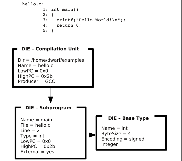
例如下图中就展示了一个简单的程序的DWARF信息:
image.png
最上面的是CU编译单元,它作为DWARF信息的根节点,包含了两个下级DIE。其中一个描述main的信息,如返回类型、行号、函数起始地址…另一个DIE描述的是int类型,通过子程序DIE中的Type属性而被引用。
DIE类型
DIE可以分为两种通用类型:
一类用来描述数据的DIE
另一类用来描述函数或者其他可执行代码
基础类型->数据类型
大多数语言都有复杂的数据类型体系,例如内置数据类型、指针、数据结构、自定义结构等类型。这些基于语言底层设计的主要类型我们称之为基础类型 ,其他的数据类型都由这些基础类型构造而成。
一个具名变量由一个拥有多种属性的 DIE
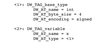
描述,其中一个属性是对类型定义的引用。下图就描述了一个名为x的整型变量:
image.png
int
的基础类型将其描述为一个占用四个字节的有符号二进制整数。用于变量
x 的 DW_TAG_variable DIE
给出了它的名称和一个类型属性,该属性引用了基础类型 DIE。
同样的,DWARF
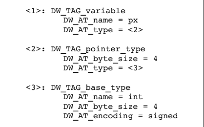
也可以使用基础类型通过组合来构建其他数据类型定义。一个新类型是作为对另一个类型的补充而创建的。以下面这个int* px的DIE信息为例:
image.png
这个 DIE 定义了一个指针类型,指明其大小为四个字节,并继而引用了
int 基础类型。
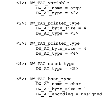
还可以更复杂的,比如加上关键词去限定这个变量的属性和类型,也可以将更多类型的DIE链接在一起以描述更复杂的数据类型,例如const char ** argv的DIE信息如下:
image.png
总的来说,在DWARF信息中,我们通过组合基本类型的方式来表示程序语言中的数据类型。这样我们无需了解所有程序语言的数据结构,也可以描述出数据类型的信息。
常见类型
数组
数组类型由DW_TAG_array_type表示,对于int arr[10],其一般DWARF结构如下:
1 2 3 4 5 6 7 8 9 10 11 12 13 14 15 16 17 18 19 20 21 22 23 < 1 ><0x0000002e > DW_TAG_array_type DW_AT_type <0x00000045 > DW_AT_sibling <0x0000003e > < 2 ><0x00000037 > DW_TAG_subrange_type DW_AT_type <0x0000003e > DW_AT_upper_bound 9 < 1 ><0x0000003e > DW_TAG_base_type DW_AT_byte_size 0x00000008 DW_AT_encoding DW_ATE_unsigned DW_AT_name long unsigned int < 1 ><0x00000045 > DW_TAG_base_type DW_AT_byte_size 0x00000004 DW_AT_encoding DW_ATE_signed DW_AT_name int < 1 ><0x0000004c > DW_TAG_variable DW_AT_name arr DW_AT_decl_file 0x00000001 /home/ylin/Program/test/./test.c DW_AT_decl_line 0x00000001 DW_AT_decl_column 0x00000005 DW_AT_type <0x0000002e > DW_AT_external yes (1 ) DW_AT_location len 0x0009: 0x034040000000000000: DW_OP_addr 0x00004040
其中DW_TAG_subrange_type用来存储描述数组维度的范围(下标范围),这里不仅指示了下标的上界DW_AT_upper_bound 9也指明了下标的数据类型DW_AT_type <0x0000003e>
我们可以看到左边的<1> <2>的符号,这代表当前条目在条目树结构中的深度。
理解了数据类型的结构分析之后,我们看到变量的定义信息:
DW_AT_name:变量名
DW_AT_decl_line:变量的定义行
DW_AT_decl_column:变量的定义列
DW_AT_type:变量定义类型
DW_AT_external:变量的作用域范围(全局符号)
DW_AT_location:变量在内存中的存储位置
通过这些信息,我们就可以还原出数组的数据类型、存储结构、以及在源代码中的定义位置等信息
结构、类、联合体、接口
大多数的语言都支持将各种数据类型的组合到一个结构体中,只不过不同的语言叫法不一样而已,这里的我们就简单的介绍一下结构体和类的标签。
结构体相较于类更加纯粹,它主要对数据进行封装,将不同的数据类型整合成一个大的结构体,在结构体中通过字段对这些数据进行索引,我们可以看下它的DWARF结构
1 2 3 4 5 6 7 8 9 10 11 12 13 14 15 16 17 18 19 20 21 22 23 24 25 26 27 28 29 30 31 32 33 34 35 36 37 38 39 40 < 1 ><0x0000002e > DW_TAG_structure_type DW_AT_byte_size 0x00000010 DW_AT_decl_file 0x00000001 /home/ylin/Program/test/./test.c DW_AT_decl_line 0x00000001 DW_AT_decl_column 0x00000001 DW_AT_sibling <0x00000052 > < 2 ><0x00000037 > DW_TAG_member DW_AT_name age DW_AT_decl_file 0x00000001 /home/ylin/Program/test/./test.c DW_AT_decl_line 0x00000002 DW_AT_decl_column 0x00000009 DW_AT_type <0x00000052 > DW_AT_data_member_location 0 < 2 ><0x00000044 > DW_TAG_member DW_AT_name name DW_AT_decl_file 0x00000001 /home/ylin/Program/test/./test.c DW_AT_decl_line 0x00000003 DW_AT_decl_column 0x0000000b DW_AT_type <0x00000059 > DW_AT_data_member_location 8 < 1 ><0x00000052 > DW_TAG_base_type DW_AT_byte_size 0x00000004 DW_AT_encoding DW_ATE_signed DW_AT_name int < 1 ><0x00000059 > DW_TAG_pointer_type DW_AT_byte_size 0x00000008 DW_AT_type <0x0000005f > < 1 ><0x0000005f > DW_TAG_base_type DW_AT_byte_size 0x00000001 DW_AT_encoding DW_ATE_signed_char DW_AT_name char < 1 ><0x00000066 > DW_TAG_variable DW_AT_name student DW_AT_decl_file 0x00000001 /home/ylin/Program/test/./test.c DW_AT_decl_line 0x00000004 DW_AT_decl_column 0x00000002 DW_AT_type <0x0000002e > DW_AT_external yes (1 ) DW_AT_location len 0x0009: 0x032040000000000000: DW_OP_addr 0x00004020
结构体类型由DW_TAG_structure_type进行表示,这里我们定义的结构体如下:
1 2 3 4 struct { int age; char * name; }student;
我们可以阅读到以下结构体的属性:
DW_TAG_member:结构体的成员
DW_AT_data_member_location:字段在结构体中偏移值,我们可以通过这个值访问结构体中的成员
DW_AT_byte_size:结构体的大小(这里可以看出内存对齐了)
还有典型的一些属性…
然后是类的,类相当于结构体的plus版,既可以组合数据类型,也可以包含函数方法,不过对于类的内存分布,我暂时也不是很清楚。我们可以看看类的DWARF信息:
1 2 3 4 5 6 7 8 9 10 11 12 13 14 15 16 17 18 19 20 21 22 23 24 25 26 27 28 29 30 31 32 33 34 35 36 37 38 39 40 41 42 43 44 45 46 47 48 49 50 51 52 < 1 ><0x0000002a > DW_TAG_class_type DW_AT_name Student DW_AT_byte_size 0x00000010 DW_AT_decl_file 0x00000001 /home/ylin/Program/test/test.cpp DW_AT_decl_line 0x00000003 DW_AT_decl_column 0x00000007 DW_AT_sibling <0x0000006d > < 2 ><0x00000037 > DW_TAG_member DW_AT_name ID DW_AT_decl_file 0x00000001 /home/ylin/Program/test/test.cpp DW_AT_decl_line 0x00000005 DW_AT_decl_column 0x0000000d DW_AT_type <0x0000006d > DW_AT_data_member_location 0 < 2 ><0x00000043 > DW_TAG_member DW_AT_name name DW_AT_decl_file 0x00000001 /home/ylin/Program/test/test.cpp DW_AT_decl_line 0x00000008 DW_AT_decl_column 0x0000000f DW_AT_type <0x00000074 > DW_AT_data_member_location 8 DW_AT_accessibility DW_ACCESS_public < 2 ><0x00000051 > DW_TAG_subprogram DW_AT_external yes (1 ) DW_AT_name getID DW_AT_decl_file 0x00000001 /home/ylin/Program/test/test.cpp DW_AT_decl_line 0x00000009 DW_AT_decl_column 0x0000000d DW_AT_linkage_name _ZN7Student5getIDEv DW_AT_type <0x0000006d> DW_AT_accessibility DW_ACCESS_public DW_AT_declaration yes (1 ) DW_AT_object_pointer <0x00000066> < 3><0x00000066> DW_TAG_formal_parameter DW_AT_type <0x00000080> DW_AT_artificial yes (1 ) < 1><0x0000006d> DW_TAG_base_type DW_AT_byte_size 0x00000004 DW_AT_encoding DW_ATE_signed DW_AT_name int < 1><0x00000074> DW_TAG_pointer_type DW_AT_byte_size 0x00000008 DW_AT_type <0x00000079> < 1><0x00000079> DW_TAG_base_type DW_AT_byte_size 0x00000001 DW_AT_encoding DW_ATE_signed_char DW_AT_name char < 1><0x00000080> DW_TAG_pointer_type DW_AT_byte_size 0x00000008 DW_AT_type <0x0000002a> < 1><0x00000085> DW_TAG_const_type DW_AT_type <0x00000080>
类的类型由DW_TAG_class_type进行表示,这里我们定义的类是这样的:
1 2 3 4 5 6 7 8 9 10 class Student { private: int ID; public: char * name; int getID () { return ID; } };
我们可以阅读以下类的信息:
DW_TAG_subprogram:这里表示这是类的一个方法,之后会详细描述一下这个标签
DW_AT_accessibility:用来指出数据和方法的成员属性(公/私),默认为私有,DW_ACCESS_public为公有
DW_AT_object_pointer:这个是隐含得参数指向this指针参数。
类由还有很多标签,但是这里不过多进行讲解。
变量
变量通常相当简单。它们有一个名称,代表一块可以存储某种值的内存(或寄存器)。变量可以包含的值的种类,以及对其修改方式的限制(例如,是否为
const),都由变量的类型来描述。
区分变量的关键在于其值的存储位置和其作用域。变量的作用域定义了变量在程序中的哪些位置是已知的,并在某种程度上由变量声明的位置决定。在
C
语言中,在函数或块内声明的变量具有函数或块作用域。在函数外声明的变量具有全局或文件作用域。这允许在不同文件中定义同名的变量而不会冲突,也允许不同的函数或编译单元引用同一个变量。
DWARF
将变量分为三类:常量 、形式参数 和变量 。
常量 用于那些语言本身包含真正具名常量的情况,例如
Ada 参数。(C 语言本身没有将常量作为语言的一部分。声明一个
const
变量只是表示你不能在没有使用显式类型转换的情况下修改变量。)形式参数 表示传递给函数的值。我们稍后再讨论这个。
大多数变量都有一个位置属性 ,用于描述变量的存储位置。
在最简单的情况下,变量存储在内存中并具有固定地址 。
但是许多变量,例如在 C
函数内声明的变量,是动态分配 的,定位它们需要进行一些(通常简单的)计算。例如,一个局部变量可能在栈上分配,定位它可能简单到只需给帧指针加上一个固定偏移量。
在其他情况下,变量可能存储在寄存器 中。
其他变量可能需要更复杂一些的计算来定位数据。作为 C++
类成员的变量可能需要更复杂的计算来确定基类在派生类中的位置。
可执行代码段:函数与子程序
这里的函数和子程序实际上是同一个东西,硬要细分的话,函数是有返回值的,而子程序没有(我们更多是利用子程序的副作用)。我们可以看一下函数会包含的DWARF信息:
1 2 3 4 5 6 7 8 9 10 11 12 13 14 15 16 17 18 19 20 21 22 23 24 25 26 27 28 29 < 1 ><0x00000065 > DW_TAG_subprogram DW_AT_external yes (1 ) DW_AT_name hello DW_AT_decl_file 0x00000001 /home/ylin/Program/test/test.c DW_AT_decl_line 0x00000001 DW_AT_decl_column 0x00000005 DW_AT_prototyped yes (1 ) DW_AT_type <0x0000005e> DW_AT_low_pc 0x00001129 DW_AT_high_pc <offset-from-lowpc> 24 <highpc: 0x00001141> DW_AT_frame_base len 0x0001: 0x9c: DW_OP_call_frame_cfa DW_AT_call_all_calls yes (1 ) < 2><0x00000083> DW_TAG_formal_parameter DW_AT_name x DW_AT_decl_file 0x00000001 DW_AT_decl_line 0x00000001 DW_AT_decl_column 0x0000000f DW_AT_type <0x0000005e> DW_AT_location len 0x0002: 0x916c: DW_OP_fbreg -20 < 2><0x0000008e> DW_TAG_formal_parameter DW_AT_name y DW_AT_decl_file 0x00000001 DW_AT_decl_line 0x00000001 DW_AT_decl_column 0x00000016 DW_AT_type <0x0000005e> DW_AT_location len 0x0002: 0x9168: DW_OP_fbreg -24
首先我们可以看到包含源代码位置信息的三元组(文件、行、列),然后是函数的高低内存范围,一般情概况下,我们默认函数的低内存地址(起始地址)为函数的入口。函数的返回类型,由类型属性指定。
这里需要注意的是DW_OP_call_frame_cfa指定的CFA0x9c。CFA就是函数执行时,其调用者的栈帧的栈顶位置,标志着一个函数栈帧的开始边界。以下图结构为例:
1 2 3 4 5 6 7 8 9 10 11 12 13 14 (高地址) +----------------------+ | ... | | main 的局部变量 | <--- main 函数的栈帧 +----------------------+ | 返回地址 | <--- [!] hello 函数的 CFA 指向这里 +----------------------+------ hello 函数栈帧的“边界” | 保存的 RBP (帧指针) | <--- 帧基址 (Frame Base) 常常指向这里 +----------------------+ | hello 的局部变量 | | ... | | 可能还有保存的寄存器 | +----------------------+ <--- 当前 RSP 指向这里(栈顶) (低地址)
在我们的示例中,DWARF信息指出DW_AT_frame_base : DW_OP_call_frame_cfa,所以这里我们的栈基址等于CFA值。基于栈基址,我们就可以对被调用栈帧中的变量进行访问。我们看到DW_AT_location的属性下,通常有DW_OP_fbreg - 偏移值的形式来计算参数在栈帧上的位置。
DWARF不定义函数的调用约定,这一部分有应用程序二进制接口规范确定(ABI)
编译单元
大多数的程序室友多个文件构成的,每个文件会被独立编译,然后与系统库链接成最终的程序,DWARF将每个独立编译的源文件称为一个编译单元
每个编译单元的DWARF数据,都会从一个编译单元调试信息项开始。该调试信息项包含编译过程中的通用信息
1 2 3 4 5 6 7 8 < 0 ><0x0000000c > DW_TAG_compile_unit DW_AT_producer GNU C17 13.3 .0 -mtune=generic -march=x86-64 -g -O0 -fasynchronous-unwind-tables -fstack-protector-strong -fstack-clash-protection -fcf-protection DW_AT_language DW_LANG_C11 DW_AT_name test.c DW_AT_comp_dir /home/ylin/Program/test DW_AT_low_pc 0x00001129 DW_AT_high_pc <offset-from-lowpc> 61 <highpc: 0x00001166 > DW_AT_stmt_list 0x00000000
包括:
编译器和编译参数
源文件的目录路径和文件名称
编译单元在内存中的起始结束地址(如果编译单元在内存中是连续的)
编译单元占用内存的地址列表(如果编译单元在内存中非连续)
指向调试器行号的指针(DW_AT_stmt_list)
编译单元调试信息项是所有该编译单元调试信息的父项。一般情况下,调试信息会先描述数据类型,接着是全局数据,然后再是子函数。
至此基本的DWARF信息就介绍到这里。