0%

78:初窥深度学习(4)

我们先前实现了卷积神经网络的各层,以及基本的前向传播,现在我们要进一步的完善整个神经网络,通过反向传播实现对权重的更新,从而提高神经网络的准确性。

反向传播

现在我们已经完成了神经网络的前向传播,现在我们需要对每个层进行反向传播以更新权重,来寻来你神经网络。进行反向传播,我们需要注意两点:

  • 在前向传播的阶段,我们需要在每一层换从它需要用于反向传播的数据(如中间值等)。这也反映了,任意反向传播的阶段,都需要有着相应的前向阶段。
  • 在反向传播阶段,每一层都会接受一个梯度,并返回一个梯度。其接受其输出($\frac{\partial L}{\partial out}$)的损失梯度,并返回其输入($\frac{\partial L}{\partial in}$)的损失梯度

我们的训练过程应该是这样的:

1
2
3
4
5
6
7
8
9
10
11
12
13
# 前向传播
out = conv.forward((image / 255) - 0.5)
out = pool.forward(out)
out = softmax.forward(out)

# 初始化梯度
gradient = np.zeros(10)
# ...

# 反向传播
gradient = softmax.backprop(gradient)
gradient = pool.backprop(gradient)
gradient = conv.backprop(gradient)

现在我们将逐步构建我们的反向传播函数:

Softmax层反向传播

我们的损失函数是: $$ \begin{align*} L = -ln(p_c) \end{align*} $$ 所以我们首先要计算的就是对于softmax层反向传播阶段的输入,其中out_s就是softmax层的输出。一个包含了10个概率的向量,我们只在乎正确类别的损失,所以我们的第一个梯度为: $$ \begin{align*} \frac{\partial L}{\partial out_s(i)} = \begin{cases} 0 \space\space\space\space\space \text{ if i!=c} \\ -\frac{1}{p_i} \text{ if i=c} \end{cases} \end{align*} $$ 所以我们正确的初始梯度应该是:

1
2
gradient = np.zeros(10)
gradient[label] = -1 / out[label]

然后我们对softmax层的前向传播阶段进行一个缓存:

1
2
3
4
5
6
7
8
9
10
11
12
13
def forward(self, input):
# 输入体积的形状
self.last_input_shape = input.shape
input = input.flatten()
# 展平后的输入向量
self.last_input = input

totals = np.dot(input,self.weights) + self.biases
# 输出结果(提供给激活函数)
self.last_totals = totals
exp = np.exp(totals)

return exp/np.sum(exp,axis=0)

现在我们可以开始准备softmax层的反向传播了:

计算

我们已经计算出,损失对于激活函数值的梯度,我们现在需要进一步的推导,最终我们希望得到$\frac{\partial L}{\partial input} \frac{\partial L}{\partial w} \frac{\partial L}{\partial b}$

的梯度,以用于对权重的梯度训练。根据链式法则,我们应该有: $$ \begin{align*} \frac{\partial L}{\partial w} &= \frac{\partial L}{\partial out} * \frac{\partial out}{\partial t} * \frac{\partial t}{\partial w} \\ \frac{\partial L}{\partial b} &= \frac{\partial L}{\partial out} * \frac{\partial out}{\partial t} * \frac{\partial t}{\partial b} \\ \frac{\partial L}{\partial input} &= \frac{\partial L}{\partial out} * \frac{\partial out}{\partial t} * \frac{\partial t}{\partial input} \end{align*} $$ 其中 t = w * input + bout则是softmax函数的输出值,我们可以依次求出。对于$\frac{\partial L}{\partial out}$我们有: $$ \begin{align*} out_s(c) &= \frac{e^{t_c}}{\sum_{i}e^{t_i}} = \frac{e^{t_c}}{S} \\ S &= \sum_{i}e^{t_i} \\ \to out_s(c) &= e^{t_c}S^{-1} \end{align*} $$ 现在我们求$\frac{\partial out_s(c)}{\partial t_k}$,需要分别考虑k=ck!=c的情况,我们依次进行求导: $$ \begin{align*} \frac{\partial out_s(c)}{\partial t_k} &= \frac{\partial out_s(c)}{\partial S} *\frac{\partial S}{\partial t_k} \\ &= -e^{t_c}S^{-2}\frac{\partial S}{\partial t_k} \\ &= -e^{t_c}S^{-2}(e^{t_k}) \\ &= \frac{-e^{t_c}e^{t_k}}{S^2} \\ \\ \frac{\partial out_s(c)}{\partial t_c} &= \frac{Se^{t_c}-e^{t_c}\frac{\partial S}{\partial t_c}}{S^2} \\ &= \frac{Se^{t_c}-e^{t_c}e^{t_c}}{S^2} \\ &= \frac{e^{t_c}(S-e^{t_c})}{S^2} \\ \to \frac{\partial out_s(k)}{\partial t} &= \begin{cases} \frac{-e^{t_c}e^{t_k}}{S^2} \space\space\space\space \text{ if k!=c} \\ \frac{e^{t_c}(S-e^{t_c})}{S^2} \text{ if k=c} \end{cases} \end{align*} $$ 最后我们根据公式t = w * input + b得到: $$ \begin{align*} \frac{\partial t}{\partial w}&=input \\ \frac{\partial t}{\partial b}&=1 \\ \frac{\partial t}{\partial input}&=w \end{align*} $$ 现在我们可以用代码实现这个过程了

实现

1
2
3
4
5
6
7
8
9
10
11
12
13
14
15
16
17
18
19
20
21
22
23
24
25
26
27
28
29
30
def backprop(self,d_L_d_out):
# d_L_d_out是这一层的输出梯度,作为参数
# 返回d_L_d_in作为下一层的参数
for i,gradient in enumerate(d_L_d_out):
if gradient == 0:
continue
# e^totals
t_exp = np.exp(self.last_totals)
# S = sum(e^totals)
S = np.sum(t_exp)
# total对out[i]的梯度关系
# 第一次是对所有的梯度进行更新
d_out_d_t = -t_exp[i]*t_exp / (S**2)
# 第二次是只对 =i 的梯度进行更新 从而使第一次的更新只针对 !=i 的梯度
d_out_d_t[i] = t_exp[i]*(S-t_exp[i]) / (S**2)
# 权重对total的梯度关系
d_t_d_w = self.last_input
d_t_d_b = 1
d_t_d_input = self.weights
# total对Loss的梯度关系
d_L_d_t = gradient * d_out_d_t
# 权重对Loss的梯度关系
d_L_d_w = d_t_d_w[np.newaxis].T @ d_L_d_t[np.newaxis]
d_L_d_b = d_L_d_t * d_t_d_b
d_L_d_input = d_t_d_input @ d_L_d_t
# 梯度训练
self.weights -= self.learn_rate * d_L_d_w
self.biases -= self.learn_rate * d_L_d_b
# 返回梯度
return d_L_d_input.reshape(self.last_input_shape)

由于softmax层的输入是一个输入体积,在一开始被我们展平处理了,但是我们返回的梯度也应该是一个同样大小的输入体积,所以我们需要通过reshape确保这层的返回的梯度和原始的输入格式相同。

我们可以测试一下softmax反向传播后的训练效果:

1
2
3
4
5
6
7
8
9
10
11
12
13
14
15
16
17
18
19
20
21
22
23
24
25
26
27
28
29
30
31
32
33
34
35
36
37
38
39
40
41
42
43
44
45
46
47
48
49
50
import numpy as np

from conv import Conv3x3
from maxpool import MaxPool2
from softmax import Softmax
import tensorflow as tf

(x_train, y_train), (x_test, y_test) = tf.keras.datasets.mnist.load_data()

test_images = x_test[:1000]
test_labels = y_test[:1000]

conv = Conv3x3(8)
pool = MaxPool2()
softmax = Softmax(13*13*8,10)

def forward(image,label):
out = conv.forward((image / 255) - 0.5)
out = pool.forward(out)
out = softmax.forward(out)

loss = -np.log(out[label])
acc = 1 if np.argmax(out) == label else 0

return out,loss,acc

def train(image,label):
out, loss, acc = forward(image,label)
gradient = np.zeros(10)
gradient[label] = -1 / out[label]
gradient = softmax.backprop(gradient)

return loss,acc

print("Start!")
loss = 0
num_correct = 0

for i,(im,label) in enumerate(zip(test_images,test_labels)):
_, l, acc = forward(im,label)
if i%100 == 99:
print(
'[Step %d] Past 100 steps :Average Loss %.3f | Accuracy %d%%' %
(i+1,loss/100,num_correct)
)
loss = 0
num_correct = 0
l,acc = train(im,label)
loss += l
num_correct += acc

可以看到准确率有明显的提升,说明我们softmax层的反向传播在很好的进行

1
2
3
4
5
6
7
8
9
10
11
Start!
[Step 100] Past 100 steps :Average Loss 2.112 | Accuracy 24%
[Step 200] Past 100 steps :Average Loss 1.940 | Accuracy 37%
[Step 300] Past 100 steps :Average Loss 1.686 | Accuracy 50%
[Step 400] Past 100 steps :Average Loss 1.606 | Accuracy 51%
[Step 500] Past 100 steps :Average Loss 1.451 | Accuracy 58%
[Step 600] Past 100 steps :Average Loss 1.362 | Accuracy 65%
[Step 700] Past 100 steps :Average Loss 1.264 | Accuracy 66%
[Step 800] Past 100 steps :Average Loss 1.057 | Accuracy 75%
[Step 900] Past 100 steps :Average Loss 0.978 | Accuracy 81%
[Step 1000] Past 100 steps :Average Loss 0.966 | Accuracy 78%

池化层传播

在前向传播的过程中,最大池化层接收一个输入体积,然后通过2x2区域的最大池化,将宽度和高度都减半。而在反向传播中,执行相反的操作:我们将损失梯度的宽度和高度都翻倍,通过将每个梯度值分配到对应的2x2区域的最大值位置:

image.png

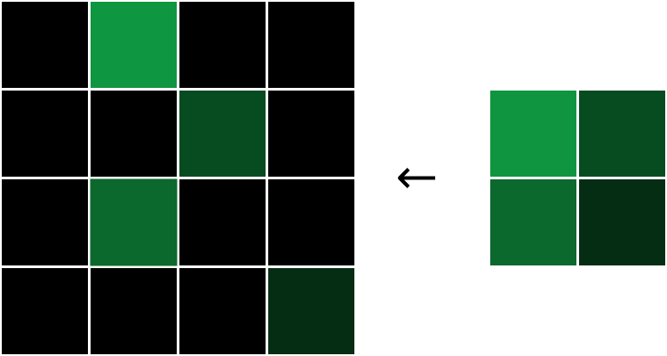
每个梯度都被分配到原始最大值的位置,然后将其他梯度设置为0.

为什么是这这样的呢?在一个2x2区域中,由于我们只关注区域内的最大值,所以对于其他的非最大值,我们可以几乎忽略不计,因为它的改变对我们的输出结果没有影响,所以对于非最大像素,我们有$\frac{\partial L}{\partial inputs}=0$。另一方面来看,最大像素的$\frac{\partial output}{\partial input}=1$,这意味着$\frac{\partial L}{\partial output}=\frac{\partial L}{\partial input}$

所以对于这一层的反向传播,我们只需要简单的还原,并且填充梯度值到最大像素区域就行了

实现

1
2
3
4
5
6
7
8
9
10
11
12
13
14
def backprop(self,d_L_d_out):
# 这里的self.last_input是前向阶段的数据缓存
d_L_d_input = np.zeros(self.last_input.shape)
for im_region,i,j in self.iterate_regions(self.last_input):
h,w,f = im_region.shape
amax = np.amax(im_region,axis=(0,1))

for i2 in range(h):
for j2 in range(w):
for f2 in range(f):
# 搜寻区域内的最大值并赋梯度值
if im_region[i2,j2,f2] == amax[f2]:
d_L_d_input[i*2+i2, j*2+j2,f2] = d_L_d_out[i,j,f2]
return d_L_d_input

这一部分并没有什么权重用来训练,所以只是一个简单的数据还原。

卷积层反向传播

卷积层的反向传播,我们需要的是卷积层中的滤波器的损失梯度,因为我们需要利用损失梯度来更新我们滤波器的权重,我们现在已经有了$\frac{\partial L}{\partial output}$,我们现在只需要计算$\frac{\partial output}{\partial filters}$,所以我们需要知道,改变一个滤波器的权重会怎么影响到卷积层的输出?

实际上修改滤波器的任意权重都可能会导致滤波器输出的整个图像,下面便是很好的示例:

image.png
image.png

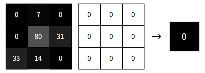
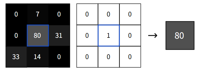
同样的对任何滤波器权重+1都会使输出增加相应图像像素的值,所以输出像素相对于特定滤波器权重的导数应该就是相应的图像元素。我们可以通过数学计算来论证这一点

计算

$$ \begin{align*} out(i,j) &= convolve(image,filiter) \\ &= \sum_{x=0}^3{}\sum_{y=0}^{3}image(i+x,j+y)*filiter(x,y) \\ \to \frac{\partial out(i,j)}{\partial filiter(x,y)} &=image(i+x,i+y) \end{align*} $$

我们将输出的损失梯度引进来,我们就可以获得特定滤波器权重的损失梯度了: $$ \begin{align*} \frac{\partial L}{\partial filiter(x,y)} = \sum_{i}\sum_{j}\frac{\partial L}{\partial out(i,j)} * \frac{\partial out(i,j)}{\partial filter(x,y)} \end{align*} $$ 现在我们可以实现我们卷积层的反向传播了:

实现

1
2
3
4
5
6
7
8
9
def backprop(self, d_L_d_out):
d_L_d_filters = np.zeros(self.filters.shape)

for im_region, i, j in self.iterate_regions(self.last_input):
for f in range(self.num_filters):
d_L_d_filters[f] += d_L_d_out[i, j, f] * im_region

self.filters -= self.learn_rate * d_L_d_filters
return None

现在我们可以对我们的神经网络进行一个完整的训练了,我们可以看到训练的结果如下:
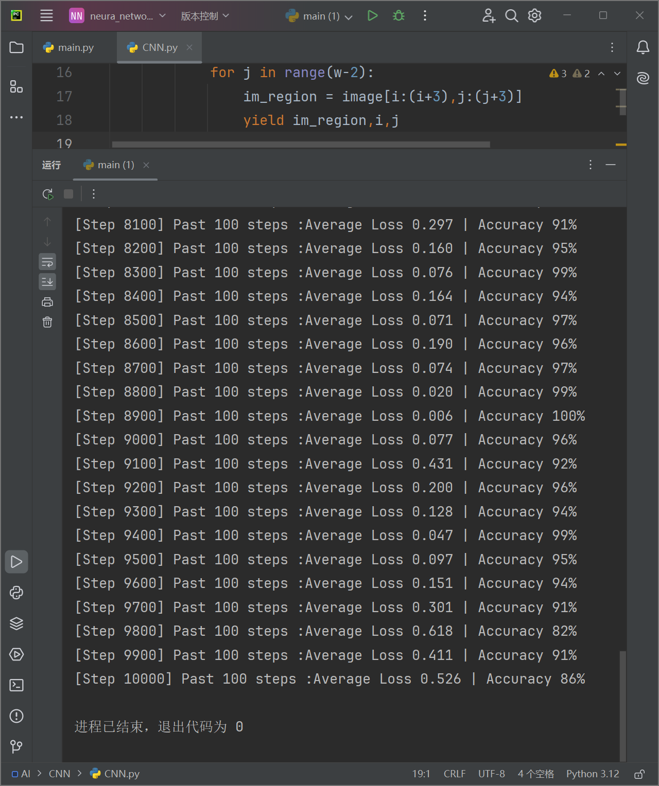
image.png

效果还是非常不错的。

完善

和之前的网络不同,CNN的训练集比较庞大,如果每次启动都要训练遍参数就太麻烦了,所以我们可以再每次训练之后将参数保存下来。下次再要使用就可以直接加载而不用重复训练。所以我们可以编写保存模型:

1
2
3
4
5
6
7
8
9
10
11
12
13
14
15
16
17
18
19
20
21
22
23
24
25
26
27
28
29
30
31
32
import pickle

class ModelSaver:
def __init__(self, model_name='MNIST_CNN'):
self.model_name = model_name

def save(self, conv, pool, softmax):
data = {
'conv_filters': conv.filters,
'softmax_weights': softmax.weights,
'softmax_biases': softmax.biases
}
filename = f'{self.model_name}.pkl'
with open(filename, 'wb') as f:
pickle.dump(data, f)
print(f"保存参数到{filename}")

def load(self, conv, pool, softmax):
filename = f'{self.model_name}.pkl'
try:
with open(filename, 'rb') as f:
data = pickle.load(f)

conv.filters = data['conv_filters']
softmax.weights = data['softmax_weights']
softmax.biases = data['softmax_biases']
print("模型参数加载成功")
return True

except FileNotFoundError:
print("无可用模型参数")
return False

如果我们想要自己尝试手写输入,来测试模型的效果,我们可能希望有个手写板,所以我们可以再写一个手写板的类:

1
2
3
4
5
6
7
8
9
10
11
12
13
14
15
16
17
18
19
20
21
22
23
24
25
26
27
28
29
30
31
32
33
34
35
36
37
38
39
40
41
42
43
44
45
46
47
48
49
50
51
52
53
54
55
class DrawingBoard:
def __init__(self, root):
self.root = root
self.root.title("画板")

# 创建一个 Canvas 作为画板
self.canvas = tk.Canvas(root, width=280, height=280, bg='white')
self.canvas.pack()

# 绑定鼠标事件
self.canvas.bind("<B1-Motion>", self.paint)

# 初始化绘图工具
self.image = Image.new("RGB", (280, 280), "white")
self.draw = ImageDraw.Draw(self.image)

# 初始化画笔颜色和宽度
self.brush_color = "black"
self.brush_width = 5

# 添加输出按钮
self.output_button = tk.Button(root, text="输出", command=self.output_and_exit)
self.output_button.pack()

def paint(self, event):
x1, y1 = (event.x - self.brush_width), (event.y - self.brush_width)
x2, y2 = (event.x + self.brush_width), (event.y + self.brush_width)
self.canvas.create_oval(x1, y1, x2, y2, fill=self.brush_color, outline=self.brush_color)
self.draw.ellipse([x1, y1, x2, y2], fill=self.brush_color, outline=self.brush_color)

def process_image(self):
# 将图像调整为 28x28 像素
processed_image = self.image.resize((28, 28), Image.Resampling.LANCZOS)
processed_image = ImageOps.grayscale(processed_image)

# 将图像转换为 NumPy 数组
image_array = np.array(processed_image)

# 确保像素值是整数
image_array = image_array.astype(np.uint8)

return image_array

def output_and_exit(self):
# 处理图像并获取数组
self.image_array = self.process_image()

# 保存图像
processed_image = Image.fromarray(self.image_array)
processed_image.save("temp.png")
print("图片已保存为 temp.png")

# 退出程序
self.root.destroy()

现在我们就可以使用它了,我们先进行训练,然后用保存的参数,来进行手写数字识别,我把整个网络的源代码放在下面:

1
2
3
4
5
6
7
8
9
10
11
12
13
14
15
16
17
18
19
20
21
22
23
24
25
26
27
28
29
30
31
32
33
34
35
36
37
38
39
40
41
42
43
44
45
46
47
48
49
50
51
52
53
54
55
56
57
58
59
60
61
62
63
64
65
66
67
68
69
70
71
72
73
74
75
76
77
78
79
80
81
82
83
84
85
86
87
88
89
90
91
92
93
94
95
96
97
98
99
100
101
102
103
104
105
106
107
108
109
110
111
112
113
114
115
116
117
118
119
120
121
122
123
124
125
126
127
128
129
130
131
132
133
134
135
136
137
138
139
140
141
142
143
144
145
146
147
148
149
150
151
152
153
154
155
156
157
158
159
160
161
162
163
164
165
166
167
168
169
170
171
172
173
174
175
176
177
178
179
180
181
182
183
184
185
186
187
188
189
190
191
192
193
194
195
196
197
198
199
200
201
202
203
204
205
206
207
208
209
210
211
212
213
214
215
216
217
218
219
220
221
222
223
224
225
226
227
228
import numpy as np

class Conv3x3:
# 使用3x3滤波器的卷积层
def __init__(self, num_filters, learn_rate=0.01):
self.num_filters = num_filters
self.filters = np.random.randn(num_filters, 3, 3) / 9

self.last_input = None
self.learn_rate = learn_rate

def iterate_regions(self, image):
# 返回所有可以卷积的3x3的图像区域
h, w = image.shape
for i in range(h - 2):
for j in range(w - 2):
im_region = image[i:(i + 3), j:(j + 3)]
yield im_region, i, j

def forward(self, input):
# 执行卷积层的前向传播 输出一个26x26x8的三维输出数组
self.last_input = input
h, w = input.shape
output = np.zeros((h - 2, w - 2, self.num_filters))
for im_region, i, j in self.iterate_regions(input):
output[i, j] = np.sum(im_region * self.filters, axis=(1, 2))

return output

def backprop(self, d_L_d_out):
d_L_d_filters = np.zeros(self.filters.shape)

for im_region, i, j in self.iterate_regions(self.last_input):
for f in range(self.num_filters):
d_L_d_filters[f] += d_L_d_out[i, j, f] * im_region

self.filters -= self.learn_rate * d_L_d_filters

return None


class MaxPool2:
# 池化尺寸为2的最大池化层
def __init__(self):
self.last_input = None

def iterate_regions(self, image):
h, w, _ = image.shape
new_h = h // 2
new_w = w // 2

for i in range(new_h):
for j in range(new_w):
im_region = image[i * 2:(i + 1) * 2, j * 2:(j + 1) * 2]
yield im_region, i, j

def forward(self, input):
self.last_input = input
h, w, num_filters = input.shape
output = np.zeros((h // 2, w // 2, num_filters))

for im_region, i, j in self.iterate_regions(input):
output[i, j] = np.amax(im_region, axis=(0, 1))

return output

def backprop(self, d_L_d_out):
d_L_d_input = np.zeros(self.last_input.shape)
for im_region, i, j in self.iterate_regions(self.last_input):
h, w, f = im_region.shape
amax = np.amax(im_region, axis=(0, 1))

for i2 in range(h):
for j2 in range(w):
for f2 in range(f):
if im_region[i2, j2, f2] == amax[f2]:
d_L_d_input[i * 2 + i2, j * 2 + j2, f2] = d_L_d_out[i, j, f2]
return d_L_d_input


class Softmax:
# 全连接softmax激活层
def __init__(self, input_len, nodes, learn_rate=0.01):
self.weights = np.random.randn(input_len, nodes) / nodes
self.biases = np.zeros(nodes)
self.learn_rate = learn_rate

self.last_input_shape = None
self.last_input = None
self.last_totals = None

def forward(self, input):
self.last_input_shape = input.shape
input = input.flatten()
self.last_input = input

totals = np.dot(input, self.weights) + self.biases
self.last_totals = totals
exp = np.exp(totals)

return exp / np.sum(exp, axis=0)

def backprop(self, d_L_d_out):
# d_L_d_out是这一层的输出梯度,作为参数
# 返回d_L_d_in作为下一层的参数
d_L_d_w = np.zeros(self.weights.shape)
d_L_d_b = np.zeros(self.biases.shape)
d_L_d_input = np.zeros(self.last_input.shape)
for i, gradient in enumerate(d_L_d_out):
if gradient == 0:
continue
# e^totals
t_exp = np.exp(self.last_totals)
# S = sum(e^totals)
S = np.sum(t_exp)
# total对out[i]的梯度关系
# 第一次是对所有的梯度进行更新
d_out_d_t = -t_exp[i] * t_exp / (S ** 2)
# 第二次是只对 =i 的梯度进行更新 从而使第一次的更新只针对 !=i 的梯度
d_out_d_t[i] = t_exp[i] * (S - t_exp[i]) / (S ** 2)
# 权重对total的梯度关系
d_t_d_w = self.last_input
d_t_d_b = 1
d_t_d_input = self.weights
# total对Loss的梯度关系
d_L_d_t = gradient * d_out_d_t
# 权重对Loss的梯度关系
d_L_d_w += d_t_d_w[np.newaxis].T @ d_L_d_t[np.newaxis]
d_L_d_b += d_L_d_t * d_t_d_b
d_L_d_input += d_t_d_input @ d_L_d_t
# 梯度训练
self.weights -= self.learn_rate * d_L_d_w
self.biases -= self.learn_rate * d_L_d_b
# 返回梯度
return d_L_d_input.reshape(self.last_input_shape)


import pickle

class ModelSaver:
def __init__(self, model_name='MNIST_CNN'):
self.model_name = model_name

def save(self, conv, pool, softmax):
data = {
'conv_filters': conv.filters,
'softmax_weights': softmax.weights,
'softmax_biases': softmax.biases
}
filename = f'{self.model_name}.pkl'
with open(filename, 'wb') as f:
pickle.dump(data, f)
print(f"保存参数到{filename}")

def load(self, conv, pool, softmax):
filename = f'{self.model_name}.pkl'
try:
with open(filename, 'rb') as f:
data = pickle.load(f)

conv.filters = data['conv_filters']
softmax.weights = data['softmax_weights']
softmax.biases = data['softmax_biases']
print("模型参数加载成功")
return True

except FileNotFoundError:
print("无可用模型参数")
return False


import tkinter as tk
from PIL import Image,ImageDraw,ImageOps

class DrawingBoard:
def __init__(self, root):
self.root = root
self.root.title("画板")

# 创建一个 Canvas 作为画板
self.canvas = tk.Canvas(root, width=280, height=280, bg='white')
self.canvas.pack()

# 绑定鼠标事件
self.canvas.bind("<B1-Motion>", self.paint)

# 初始化绘图工具
self.image = Image.new("RGB", (280, 280), "white")
self.draw = ImageDraw.Draw(self.image)

# 初始化画笔颜色和宽度
self.brush_color = "black"
self.brush_width = 5

# 添加输出按钮
self.output_button = tk.Button(root, text="输出", command=self.output_and_exit)
self.output_button.pack()

def paint(self, event):
x1, y1 = (event.x - self.brush_width), (event.y - self.brush_width)
x2, y2 = (event.x + self.brush_width), (event.y + self.brush_width)
self.canvas.create_oval(x1, y1, x2, y2, fill=self.brush_color, outline=self.brush_color)
self.draw.ellipse([x1, y1, x2, y2], fill=self.brush_color, outline=self.brush_color)

def process_image(self):
# 将图像调整为 28x28 像素
processed_image = self.image.resize((28, 28), Image.Resampling.LANCZOS)
processed_image = ImageOps.grayscale(processed_image)

# 将图像转换为 NumPy 数组
image_array = np.array(processed_image)

# 确保像素值是整数
image_array = image_array.astype(np.uint8)

return image_array

def output_and_exit(self):
# 处理图像并获取数组
self.image_array = self.process_image()

# 保存图像
processed_image = Image.fromarray(self.image_array)
processed_image.save("temp.png")
print("图片已保存为 temp.png")

# 退出程序
self.root.destroy()