中途歇了一段时间写物理作业，然后昨天学了下垃圾回收。现在继续开始我们的图形学学习。

漫反射材质

现在我们有了物体和每个像素的多个光线，现在我们可以尝试制作更加逼真的材质了。我们先从我们的漫反射材质开始（也称为哑光材质）开始。不过这里我们将几何体和材质分开使用，这使得我们可以将一种材质应用于多种物体，或者将多种材质应用于一种物体。这样分开使用的方法更加灵活也更加容易拓展，所以我们选择这种方式来实现我们的材质。

一个简单的漫反射材质

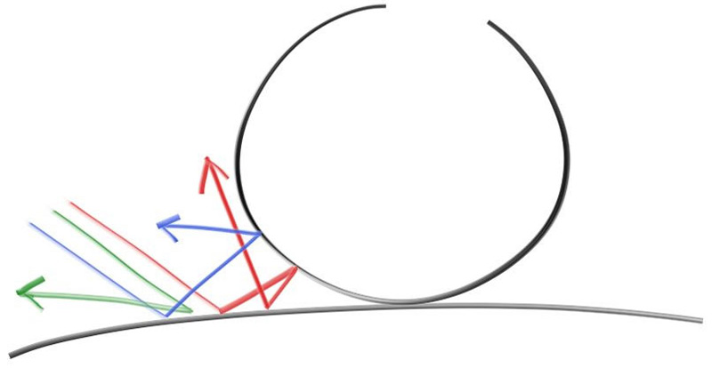
一个漫反射的物体不会发出自己的光，它会吸收周围的环境的颜色，然后通过自己固有的颜色来调节。从扩散表面反射的光线方向是随机的，我们向两个漫反射材质之间发射三束光线，他们的行为会有所不同

当然，他们有可能会被吸收，也有可能会被反射。表面越暗，说明光线被吸收的可能性更大（黑色说明光线被完全吸收了）。实际上我们我们可以用随机化方向的算法产生看起来哑光的材质，最简单的实现就是：一个光线击中表面，有相等的机会向任何方向弹射出去

这样的漫反射材质是最简单的，我们需要实现一些随机反射光线的方法，我们向vec类中再额外实现几个函数，以完成能够生成任意随机的向量：

class vec3 {
  public:
    ...

    double length_squared() const {
        return e[0]*e[0] + e[1]*e[1] + e[2]*e[2];
    }

    static vec3 random() {
        return vec3(random_double(), random_double(), random_double());
    }

    static vec3 random(double min, double max) {
        return vec3(random_double(min,max), random_double(min,max), random_double(min,max));
    }
};

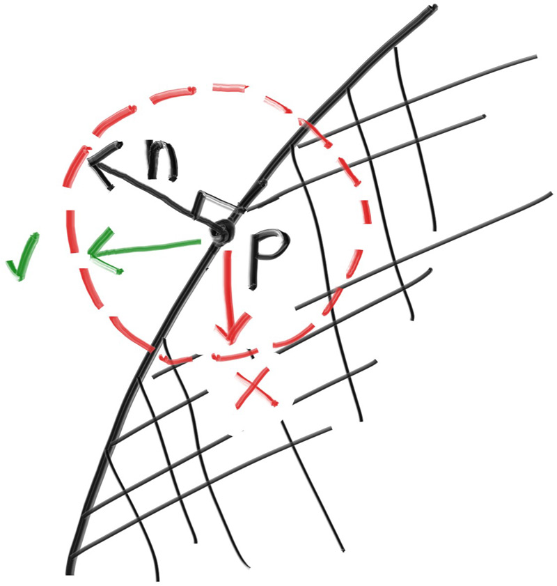
现在我们需要操作这个随机向量，以确保我们的向量生成在外半球。我们用最简单的方法来实现这个过程，即随机重复生成向量，直到生成了满足我们需求的标准样本，然后采用它，实现它的具体方法如下：

在该点的单位球体内生成一个随机向量
将这个向量单位化，以确保指向球面
如果这个向量单位化后，不在我们想要的半球，将其反转

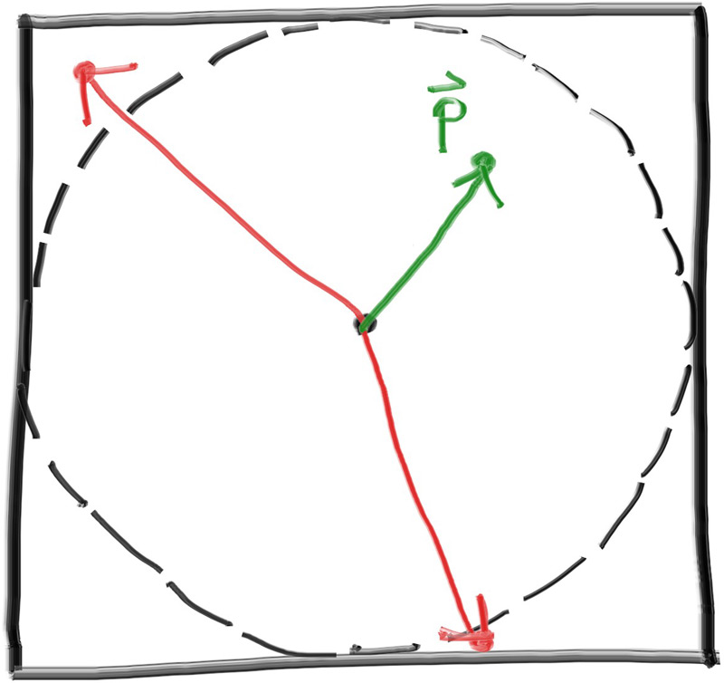
我们开始这个算法的具体实现，首先在包围单位球体的立方体内随机生成一个点(即x,y,z都在[-1,+1]内)。如果这个点在单位球体之外，则重新生成一个点，直到找到一个在单位球体内的一个点：

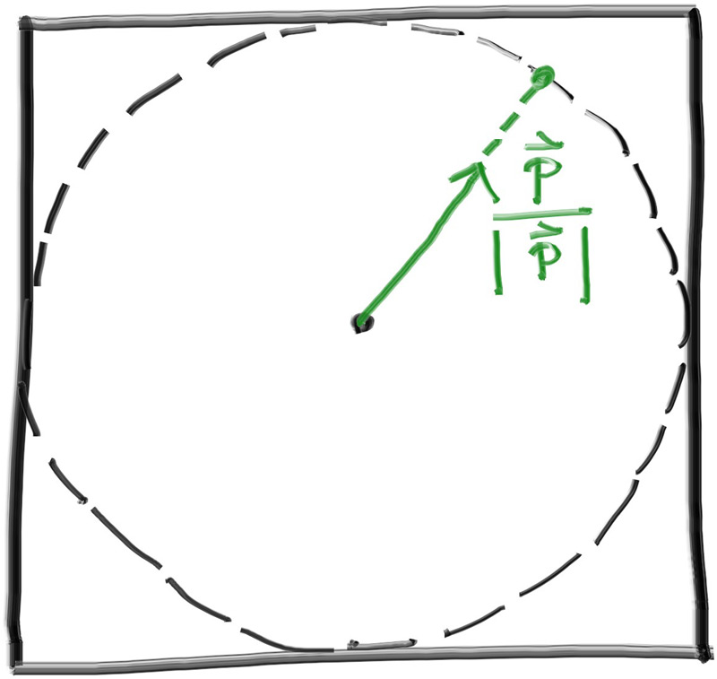
然后我们将其单位化

我们先实现这个功能吧：

//vec3.h
inline vec3 random_unit_vector(){
    while(true){
        auto p = vec3::random(-1,1);
        auto lensq = p.length_squared();
        if(lensq <= 1){
            return p/ sqrt(lensq);
        }
    }
}

实际上这里还会有一点小问题，我们需要直到。由于浮点数的精度是有限的，一个很小的数在平方后可能会向下溢出到0。也就是说，如果三个坐标都足够小（非常接近球心），向量在单位化操作下可能会变成[+-无穷,+-无穷,+-无穷]。为了解决这个问题我们需要设置一个下限值，由于我们使用的是double，所以在这里我们可以支持大于1e-160的值，所以我们更新一下程序：

//vec3.h
inline vec3 random_unit_vector(){
    while(true){
        auto p = vec3::random(-1,1);
        auto lensq = p.length_squared();
        //1e-160太极限了，所以放宽一点
        if(lensq > 1e-100 && lensq <= 1){
            return p/ sqrt(lensq);
        }
    }
}

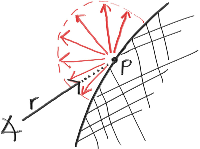
现在我们计算得到了单位球面上的随机向量，需要将其与表面法线比较，以判断其是否为位于正确的半球

//vec3.h
inline vec3 random_on_hemisphere(const vec3& normal){
    vec3 on_unit_sphere = random_unit_vector();
    if (dot(on_unit_sphere,normal) > 0.0)
        return on_unit_sphere;
    else
        return -on_unit_sphere;
}

接下来我们需要将其应用到上色函数中，这里的话我们还需要注意一点，就是光线颜色的反射率，如果反射率为100%，那么我们看到的都是白色的，如果光线反射率是0%，那么光线都被吸收，我们看到的物体是黑色的。这里我们设置我们的光线反射率为50%，并将其应用到我们的ray_color()中：

color ray_color(const ray& r, const hittable& world) const {
        hit_record rec;

        if (world.hit(r, interval(0, infinity), rec)) {
            vec3 direction = random_on_hemisphere(rec.normal);
            return 0.5 * ray_color(ray(rec.p, direction), world);
        }

        vec3 unit_direction = unit_vector(r.direction());
        auto a = 0.5*(unit_direction.y() + 1.0);
        return (1.0-a)*color(1.0, 1.0, 1.0) + a*color(0.5, 0.7, 1.0);
    }

然后我们可以看到渲染出来的图片：

限制光线的反射次数（递归深度）

注意，我们的ray_color函数是递归的，我们却不能确保它何时停止递归，也就是它不再击中任何东西的时候。当情况比较复杂的时候可能会花费很多时间或者是栈空间，为了防止这种情况我们需要限制这个程序的最大递归深度，我们将其作为camera类的一个属性，并且更改我们的ray_color()函数：

class camera{
public:
    double aspect_radio = 1.0;      //图像的宽高比
    int    image_width = 100;       //图像宽度的像素数
    int    samples_per_pixel = 10;  //每个像素的采样次数
    int    max_depth = 10;          //光线追踪的最大递归深度

    void render(const hittable& world){
        initialize();

        std::cout << "P3\n" << image_width << " " << image_height << "\n255\n";
        for(int j=0;j<image_height;j++){
            std::clog << "\rScanlines remaining: " << (image_height - j) << ' ' << std::flush;
            for(int i=0;i<image_width;i++){
                color pixel_color(0,0,0);
                for(int sample = 0;sample < samples_per_pixel; sample++){
                    ray r = get_ray(i,j);
                    pixel_color += ray_color(r,max_depth,world);
                }
                write_color(std::cout,pixel_color*pixel_samples_scale);
            }
        }
        std::clog << "\rDone.                   \n";
    }
	...
private:
	...

    color ray_color(const ray& r,int depth, const hittable& world) const {
        //如果不进行光线的追踪，就不会光线返回
        if(depth <= 0)
            return {0,0,0};

        hit_record rec;

        if (world.hit(r, interval(0, infinity), rec)) {
            vec3 direction = random_on_hemisphere(rec.normal);
            return 0.5 * ray_color(ray(rec.p, direction), depth - 1,world);
        }

        vec3 unit_direction = unit_vector(r.direction());
        auto a = 0.5*(unit_direction.y() + 1.0);
        return (1.0-a)*color(1.0, 1.0, 1.0) + a*color(0.5, 0.7, 1.0);
    }
};

同时我们可以通过更新main函数来更改我们的深度限制：

int main(){
 	...
    cam.aspect_radio = 16.0/9.0;
    cam.image_width = 800;
    cam.samples_per_pixel = 100;
    cam.max_depth = 50;

    cam.render(world);
}

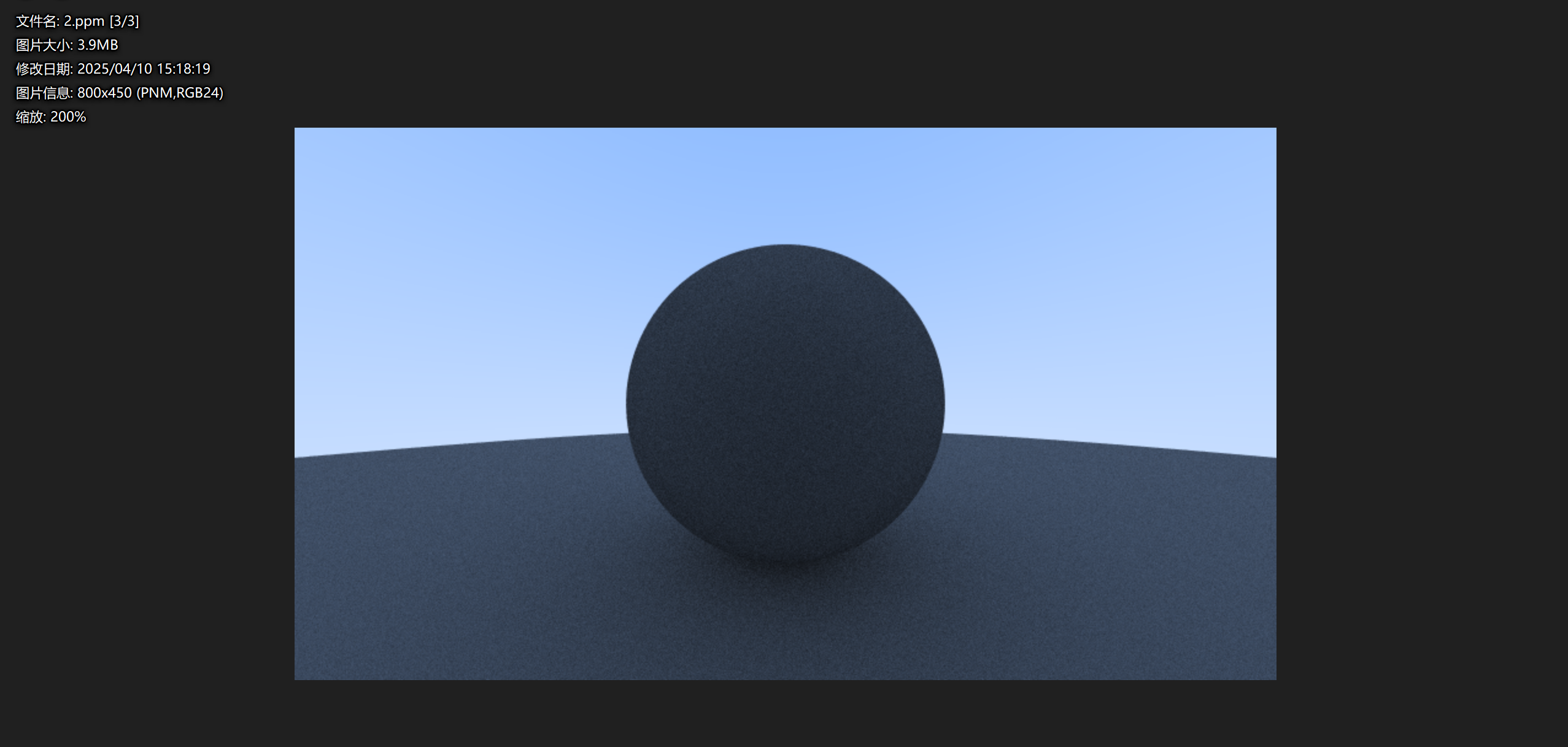
渲染出来的效果差不多

小阴影块

我们这里还需要解决一个问题，当我们计算光线与表面的交点时，计算机会尝试准确的计算出它的交点，但是由于浮点数的误差，我们很难准确的计算出来，导致交点会略微偏移，这其中就有一部分的交点会在表面之下，会导致从表面随机散射的光线再次与表面相交，可能会解出t = 0.000001,也就是在很短的距离内，再次击中表面。

所以为了解决这个问题，我们需要设置一个阈值，当t小于一定程度的时候，我们不将视作有效的命中：

color ray_color(const ray& r,int depth, const hittable& world) const {
       //如果不进行光线的追踪，就不会光线返回
       if(depth <= 0)
           return {0,0,0};

       hit_record rec;

       if (world.hit(r, interval(0.001, infinity), rec)) {
           vec3 direction = random_on_hemisphere(rec.normal);
           return 0.5 * ray_color(ray(rec.p, direction), depth - 1,world);
       }

       vec3 unit_direction = unit_vector(r.direction());
       auto a = 0.5*(unit_direction.y() + 1.0);
       return (1.0-a)*color(1.0, 1.0, 1.0) + a*color(0.5, 0.7, 1.0);
   }

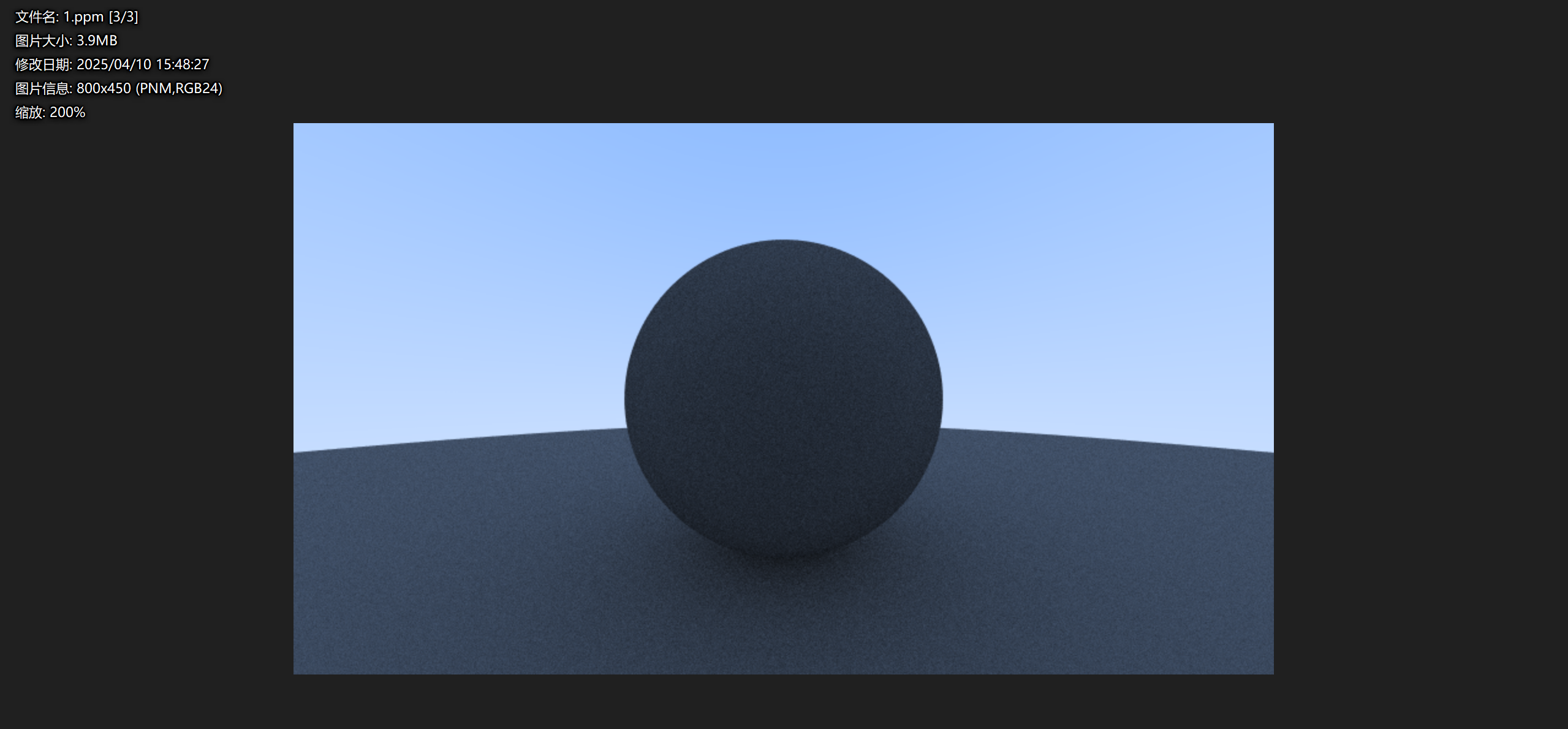
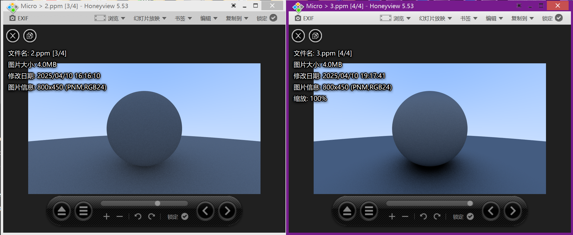
我们在此基础上再尝试渲染一次，看看效果：

右边是修复后的效果，我们可以明显感受到其变得更加明亮，更加真实

Lambertian反射

我们先前用的是随机的光线来实现漫反射，这样的话会虽然可以正确的渲染出我们的图像，但是缺少了一点真实感，在实际的漫反射中，反射光线遵循一定的规律（应该是在图形学中通常使用Lambertian定理来实现漫反射）

Lambertian反射的核心思想是反射光的亮度和观察的方向无关，而是和入射光线和表面法线的夹角有关，实际上他们之间存在I = I0*cos(/theta)的关系。

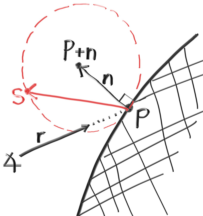
为了在光线追踪中模拟Lambertian分布，我们可以通过移动单位球的方式以实现这个过程，我们向随机生成的单位向量添加一个法向量，来实现这个移动。这么说可能比较抽象，可以看下以下图片：

我们将单位球沿着法线方向移动生成一个新的单位球，此时我们随机分布的点位是大致符合Lambertian反射的，具体的内容可以自己去尝试Lambertian分布的搜索。

这个过程看起来很复杂，实际上实现起来十分简单：

color ray_color(const ray& r,int depth, const hittable& world) const {
        //如果不进行光线的追踪，就不会光线返回
        if(depth <= 0)
            return {0,0,0};

        hit_record rec;

        if (world.hit(r, interval(0.001, infinity), rec)) {
            //我们只需要在这里添加一个法向量即可
            vec3 direction = rec.normal + random_on_hemisphere(rec.normal);
            return 0.5 * ray_color(ray(rec.p, direction), depth - 1,world);
        }

        vec3 unit_direction = unit_vector(r.direction());
        auto a = 0.5*(unit_direction.y() + 1.0);
        return (1.0-a)*color(1.0, 1.0, 1.0) + a*color(0.5, 0.7, 1.0);
    }

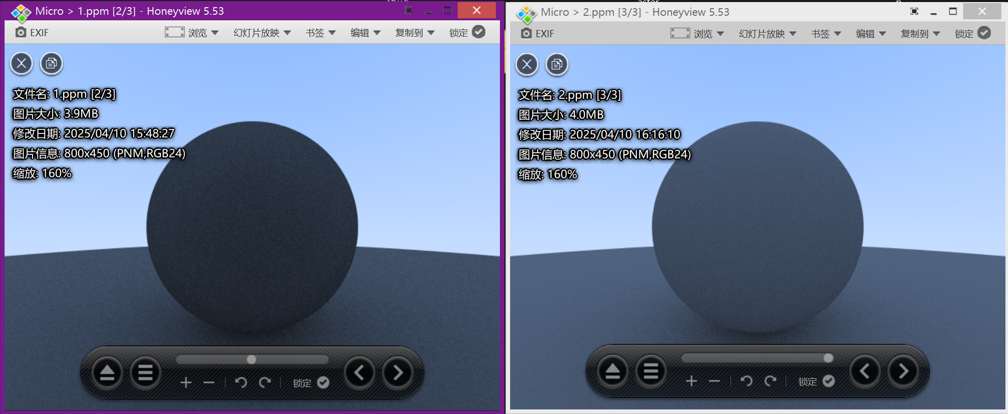
然后我们再次尝试渲染：

右图是经过Lambertian反射后生成的渲染图像，可以注意到经过Lambertian反射的设置之后，右图的阴影变得更加明显。这是因为散射的光线更多的指向法线，使其更加击中，对于交界处的光线，更多的直接向上反射了，所以在球体下方的颜色会更暗淡。

伽马矫正以实现准确的色彩强度

大多数显示设备（如显示器、电视和投影仪）的亮度输出与输入信号的关系是非线性的。这种非线性关系称为伽马（gamma），通常在2.2左右。这意味着，如果直接将线性空间（即未进行伽马校正的空间）的像素值发送到显示设备，显示出来的图像会显得比预期的要暗。

人眼对亮度的感知也是非线性的。我们的眼睛对暗部细节比亮部细节更敏感。通过伽马校正，可以使图像的亮度分布更符合人眼的感知特性，从而在视觉上获得更好的效果。

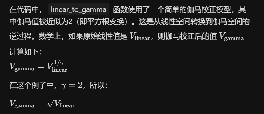
这里我们需要使用一个简单的gamma矫正模型，

我们编写我们的write_color()函数以实现从线性空间到伽马空间的变换：

inline double linear_to_gamma(double linear_component){
    if(linear_component >0)
        return std::sqrt(linear_component);
    return 0;
}

void write_color(std::ostream& out,const color& pixel_color){
    auto r = pixel_color.x();
    auto g = pixel_color.y();
    auto b = pixel_color.z();

    //从线性空间到伽马空间的转换
    r = linear_to_gamma(r);
    g = linear_to_gamma(g);
    b = linear_to_gamma(b);

    //使用区间RGB[0,1]计算RGB值
    static const interval intensity(0.000,0.999);
    int rbyte = int (256*intensity.clamp(r));
    int gbyte = int (256*intensity.clamp(g));
    int bbyte = int (256*intensity.clamp(b));

    out << rbyte << ' ' << gbyte << ' ' << bbyte << '\n';
}

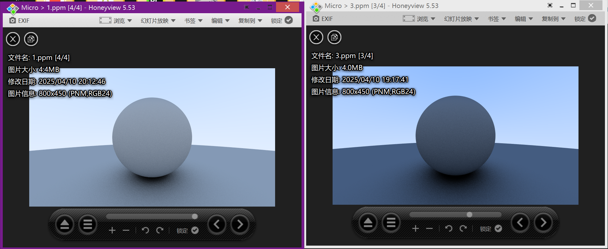
现在我们对我们的write_color()进行了伽马矫正，现在我们再来看看效果：

左边的是经过伽马矫正之后的图片，确实更好看了一点，哈哈。

Ylin's Blog

36:初始图形学(8)